AE 17: Traffic fines and electoral politics - regression with multiple predictors
Suggested answers
Last class we worked with a dataset on traffic fines revenue in California counties to investigate the question of whether or not politicians manipulate government policy during electoral years in an effort to gain an electoral advantage. We estimated a simple linear regression model with one predictor variable and found that there was not a statistically significant relationship between whether or not it is an election year and per capita traffic fines revenue. However, when we checked the assumptions of the linear model, we found that several of these assumptions were violated, casting doubt on our original results.
In this exercise we will build a series of more robust models to better evaluate the hypotheses.
The replication data file can be found in data/traffic_fines.csv. Let’s load the data and take a look at the summary statistics.1
traffic_fines <- read_csv("data/traffic_fines.csv")Rows: 1025 Columns: 95
── Column specification ────────────────────────────────────────────────────────
Delimiter: ","
chr (2): county_name, elec_dummy
dbl (93): year, county_code, vehicle_code_fines, vehicle_code_fines_i_p, she...
ℹ Use `spec()` to retrieve the full column specification for this data.
ℹ Specify the column types or set `show_col_types = FALSE` to quiet this message.skim(traffic_fines)| Name | traffic_fines |
| Number of rows | 1025 |
| Number of columns | 95 |
| _______________________ | |
| Column type frequency: | |
| character | 2 |
| numeric | 93 |
| ________________________ | |
| Group variables | None |
Variable type: character
| skim_variable | n_missing | complete_rate | min | max | empty | n_unique | whitespace |
|---|---|---|---|---|---|---|---|
| county_name | 0 | 1 | 4 | 15 | 0 | 57 | 0 |
| elec_dummy | 0 | 1 | 2 | 3 | 0 | 2 | 0 |
Variable type: numeric
| skim_variable | n_missing | complete_rate | mean | sd | p0 | p25 | p50 | p75 | p100 | hist |
|---|---|---|---|---|---|---|---|---|---|---|
| year | 0 | 1.00 | 2011.49 | 5.19 | 2003.00 | 2007.00 | 2011.00 | 2016.00 | 2020.00 | ▇▆▇▆▇ |
| county_code | 0 | 1.00 | 29.37 | 16.86 | 1.00 | 15.00 | 29.00 | 44.00 | 58.00 | ▇▇▇▇▇ |
| vehicle_code_fines | 0 | 1.00 | 1640704.86 | 3145153.92 | 0.00 | 68944.00 | 429544.00 | 1545628.00 | 21712704.00 | ▇▁▁▁▁ |
| vehicle_code_fines_i_p | 0 | 1.00 | 3.90 | 7.23 | 0.00 | 0.43 | 2.16 | 4.87 | 108.73 | ▇▁▁▁▁ |
| sheriff_incumb | 807 | 0.21 | 0.75 | 0.44 | 0.00 | 0.25 | 1.00 | 1.00 | 1.00 | ▃▁▁▁▇ |
| pre_elec | 0 | 1.00 | 1.61 | 1.11 | 0.00 | 1.00 | 2.00 | 3.00 | 3.00 | ▆▆▁▇▇ |
| no_incumb | 163 | 0.84 | 0.06 | 0.24 | 0.00 | 0.00 | 0.00 | 0.00 | 1.00 | ▇▁▁▁▁ |
| incumb | 55 | 0.95 | 0.17 | 0.37 | 0.00 | 0.00 | 0.00 | 0.00 | 1.00 | ▇▁▁▁▂ |
| sheriff_margin | 918 | 0.10 | 0.24 | 0.17 | 0.00 | 0.10 | 0.23 | 0.32 | 0.97 | ▇▇▂▁▁ |
| rep_share | 0 | 1.00 | 46.75 | 13.67 | 14.66 | 36.42 | 48.13 | 57.27 | 74.83 | ▂▅▅▇▂ |
| dem_share | 0 | 1.00 | 49.60 | 13.48 | 21.13 | 39.06 | 47.57 | 59.62 | 82.33 | ▂▇▆▅▂ |
| otherparty_share | 0 | 1.00 | 3.66 | 2.58 | 0.80 | 1.88 | 2.54 | 5.66 | 16.00 | ▇▂▂▁▁ |
| white_share | 0 | 1.00 | 57.83 | 19.31 | 12.67 | 40.35 | 56.92 | 75.99 | 89.98 | ▁▇▆▆▇ |
| asian_share | 0 | 1.00 | 6.03 | 6.70 | 0.21 | 1.27 | 3.58 | 7.04 | 32.82 | ▇▁▁▁▁ |
| black_share | 0 | 1.00 | 3.04 | 3.19 | 0.00 | 0.81 | 1.82 | 3.50 | 14.65 | ▇▂▁▁▁ |
| hispanic_share | 0 | 1.00 | 28.49 | 17.22 | 5.15 | 13.41 | 24.73 | 42.22 | 82.03 | ▇▆▃▂▁ |
| other_share | 0 | 1.00 | 4.61 | 2.93 | 1.55 | 2.89 | 3.75 | 5.52 | 21.52 | ▇▂▁▁▁ |
| young_drivers | 0 | 1.00 | 14.24 | 2.73 | 8.65 | 12.10 | 14.22 | 15.81 | 25.39 | ▅▇▅▁▁ |
| density | 0 | 1.00 | 364.64 | 694.47 | 1.53 | 24.97 | 100.92 | 321.29 | 4070.64 | ▇▁▁▁▁ |
| areain_square_miles | 0 | 1.00 | 2781.69 | 3096.29 | 440.00 | 1003.00 | 1598.00 | 3510.00 | 20164.00 | ▇▁▁▁▁ |
| med_inc | 0 | 1.00 | 55598.49 | 17114.92 | 28533.00 | 43237.00 | 52078.00 | 63398.00 | 139462.00 | ▇▇▂▁▁ |
| unemp | 0 | 1.00 | 8.72 | 3.99 | 2.10 | 5.70 | 8.00 | 10.70 | 28.90 | ▇▇▂▁▁ |
| own_source_share | 0 | 1.00 | 43.67 | 16.07 | 15.17 | 32.46 | 41.09 | 49.33 | 97.96 | ▃▇▃▁▁ |
| emp_goods | 0 | 1.00 | 43390.45 | 85018.15 | 0.00 | 2107.00 | 13093.00 | 47344.00 | 642230.00 | ▇▁▁▁▁ |
| emp_service | 0 | 1.00 | 175746.56 | 442315.84 | 0.00 | 6374.00 | 34955.00 | 124505.00 | 3439959.00 | ▇▁▁▁▁ |
| pay_goods_i | 0 | 1.00 | 39124.06 | 16100.25 | 0.00 | 29667.93 | 35001.89 | 43053.98 | 160212.25 | ▅▇▁▁▁ |
| pay_service_i | 0 | 1.00 | 31512.13 | 11371.71 | 0.00 | 25082.33 | 28896.69 | 34273.00 | 116676.48 | ▂▇▁▁▁ |
| arte_share | 56 | 0.95 | 1.75 | 2.30 | 0.00 | 0.60 | 1.11 | 1.83 | 17.49 | ▇▁▁▁▁ |
| collect_share | 56 | 0.95 | 1.75 | 1.85 | 0.00 | 0.80 | 1.22 | 1.94 | 14.79 | ▇▁▁▁▁ |
| cnty_le_sworn_1000p | 0 | 1.00 | 1.93 | 1.34 | 0.72 | 1.39 | 1.65 | 2.02 | 12.89 | ▇▁▁▁▁ |
| felony_tot_1000p | 0 | 1.00 | 12.70 | 4.58 | 4.08 | 9.48 | 11.97 | 15.49 | 34.35 | ▅▇▃▁▁ |
| misdemeanor_tot_1000p | 0 | 1.00 | 29.72 | 11.26 | 8.18 | 21.48 | 28.20 | 36.72 | 156.12 | ▇▂▁▁▁ |
| forfeitures_i_p | 0 | 1.00 | 3.34 | 6.06 | 0.00 | 0.43 | 1.98 | 4.61 | 154.06 | ▇▁▁▁▁ |
| other_court_fines_i_p | 0 | 1.00 | 10.81 | 16.44 | 0.00 | 2.79 | 6.36 | 11.62 | 154.86 | ▇▁▁▁▁ |
| delinquent_fines_i_p | 0 | 1.00 | 11.42 | 14.56 | 0.00 | 5.09 | 8.59 | 13.24 | 190.04 | ▇▁▁▁▁ |
| i_trend_1 | 0 | 1.00 | 0.17 | 1.43 | 0.00 | 0.00 | 0.00 | 0.00 | 18.00 | ▇▁▁▁▁ |
| i_trend_2 | 0 | 1.00 | 0.17 | 1.43 | 0.00 | 0.00 | 0.00 | 0.00 | 18.00 | ▇▁▁▁▁ |
| i_trend_3 | 0 | 1.00 | 0.17 | 1.43 | 0.00 | 0.00 | 0.00 | 0.00 | 18.00 | ▇▁▁▁▁ |
| i_trend_4 | 0 | 1.00 | 0.17 | 1.43 | 0.00 | 0.00 | 0.00 | 0.00 | 18.00 | ▇▁▁▁▁ |
| i_trend_5 | 0 | 1.00 | 0.17 | 1.43 | 0.00 | 0.00 | 0.00 | 0.00 | 18.00 | ▇▁▁▁▁ |
| i_trend_6 | 0 | 1.00 | 0.17 | 1.43 | 0.00 | 0.00 | 0.00 | 0.00 | 18.00 | ▇▁▁▁▁ |
| i_trend_7 | 0 | 1.00 | 0.17 | 1.43 | 0.00 | 0.00 | 0.00 | 0.00 | 18.00 | ▇▁▁▁▁ |
| i_trend_8 | 0 | 1.00 | 0.17 | 1.43 | 0.00 | 0.00 | 0.00 | 0.00 | 18.00 | ▇▁▁▁▁ |
| i_trend_9 | 0 | 1.00 | 0.17 | 1.43 | 0.00 | 0.00 | 0.00 | 0.00 | 18.00 | ▇▁▁▁▁ |
| i_trend_10 | 0 | 1.00 | 0.17 | 1.43 | 0.00 | 0.00 | 0.00 | 0.00 | 18.00 | ▇▁▁▁▁ |
| i_trend_11 | 0 | 1.00 | 0.17 | 1.43 | 0.00 | 0.00 | 0.00 | 0.00 | 18.00 | ▇▁▁▁▁ |
| i_trend_12 | 0 | 1.00 | 0.15 | 1.31 | 0.00 | 0.00 | 0.00 | 0.00 | 17.00 | ▇▁▁▁▁ |
| i_trend_13 | 0 | 1.00 | 0.17 | 1.43 | 0.00 | 0.00 | 0.00 | 0.00 | 18.00 | ▇▁▁▁▁ |
| i_trend_14 | 0 | 1.00 | 0.17 | 1.43 | 0.00 | 0.00 | 0.00 | 0.00 | 18.00 | ▇▁▁▁▁ |
| i_trend_15 | 0 | 1.00 | 0.17 | 1.43 | 0.00 | 0.00 | 0.00 | 0.00 | 18.00 | ▇▁▁▁▁ |
| i_trend_16 | 0 | 1.00 | 0.17 | 1.43 | 0.00 | 0.00 | 0.00 | 0.00 | 18.00 | ▇▁▁▁▁ |
| i_trend_17 | 0 | 1.00 | 0.17 | 1.43 | 0.00 | 0.00 | 0.00 | 0.00 | 18.00 | ▇▁▁▁▁ |
| i_trend_18 | 0 | 1.00 | 0.17 | 1.43 | 0.00 | 0.00 | 0.00 | 0.00 | 18.00 | ▇▁▁▁▁ |
| i_trend_19 | 0 | 1.00 | 0.17 | 1.43 | 0.00 | 0.00 | 0.00 | 0.00 | 18.00 | ▇▁▁▁▁ |
| i_trend_20 | 0 | 1.00 | 0.17 | 1.43 | 0.00 | 0.00 | 0.00 | 0.00 | 18.00 | ▇▁▁▁▁ |
| i_trend_21 | 0 | 1.00 | 0.17 | 1.43 | 0.00 | 0.00 | 0.00 | 0.00 | 18.00 | ▇▁▁▁▁ |
| i_trend_22 | 0 | 1.00 | 0.17 | 1.43 | 0.00 | 0.00 | 0.00 | 0.00 | 18.00 | ▇▁▁▁▁ |
| i_trend_23 | 0 | 1.00 | 0.17 | 1.43 | 0.00 | 0.00 | 0.00 | 0.00 | 18.00 | ▇▁▁▁▁ |
| i_trend_24 | 0 | 1.00 | 0.17 | 1.43 | 0.00 | 0.00 | 0.00 | 0.00 | 18.00 | ▇▁▁▁▁ |
| i_trend_25 | 0 | 1.00 | 0.17 | 1.43 | 0.00 | 0.00 | 0.00 | 0.00 | 18.00 | ▇▁▁▁▁ |
| i_trend_26 | 0 | 1.00 | 0.17 | 1.43 | 0.00 | 0.00 | 0.00 | 0.00 | 18.00 | ▇▁▁▁▁ |
| i_trend_27 | 0 | 1.00 | 0.17 | 1.43 | 0.00 | 0.00 | 0.00 | 0.00 | 18.00 | ▇▁▁▁▁ |
| i_trend_28 | 0 | 1.00 | 0.17 | 1.43 | 0.00 | 0.00 | 0.00 | 0.00 | 18.00 | ▇▁▁▁▁ |
| i_trend_29 | 0 | 1.00 | 0.17 | 1.43 | 0.00 | 0.00 | 0.00 | 0.00 | 18.00 | ▇▁▁▁▁ |
| i_trend_30 | 0 | 1.00 | 0.17 | 1.43 | 0.00 | 0.00 | 0.00 | 0.00 | 18.00 | ▇▁▁▁▁ |
| i_trend_31 | 0 | 1.00 | 0.17 | 1.43 | 0.00 | 0.00 | 0.00 | 0.00 | 18.00 | ▇▁▁▁▁ |
| i_trend_32 | 0 | 1.00 | 0.17 | 1.43 | 0.00 | 0.00 | 0.00 | 0.00 | 18.00 | ▇▁▁▁▁ |
| i_trend_33 | 0 | 1.00 | 0.17 | 1.43 | 0.00 | 0.00 | 0.00 | 0.00 | 18.00 | ▇▁▁▁▁ |
| i_trend_34 | 0 | 1.00 | 0.17 | 1.43 | 0.00 | 0.00 | 0.00 | 0.00 | 18.00 | ▇▁▁▁▁ |
| i_trend_35 | 0 | 1.00 | 0.17 | 1.43 | 0.00 | 0.00 | 0.00 | 0.00 | 18.00 | ▇▁▁▁▁ |
| i_trend_36 | 0 | 1.00 | 0.17 | 1.43 | 0.00 | 0.00 | 0.00 | 0.00 | 18.00 | ▇▁▁▁▁ |
| i_trend_37 | 0 | 1.00 | 0.17 | 1.43 | 0.00 | 0.00 | 0.00 | 0.00 | 18.00 | ▇▁▁▁▁ |
| i_trend_38 | 0 | 1.00 | 0.17 | 1.43 | 0.00 | 0.00 | 0.00 | 0.00 | 18.00 | ▇▁▁▁▁ |
| i_trend_39 | 0 | 1.00 | 0.17 | 1.43 | 0.00 | 0.00 | 0.00 | 0.00 | 18.00 | ▇▁▁▁▁ |
| i_trend_40 | 0 | 1.00 | 0.17 | 1.43 | 0.00 | 0.00 | 0.00 | 0.00 | 18.00 | ▇▁▁▁▁ |
| i_trend_41 | 0 | 1.00 | 0.17 | 1.43 | 0.00 | 0.00 | 0.00 | 0.00 | 18.00 | ▇▁▁▁▁ |
| i_trend_42 | 0 | 1.00 | 0.17 | 1.43 | 0.00 | 0.00 | 0.00 | 0.00 | 18.00 | ▇▁▁▁▁ |
| i_trend_43 | 0 | 1.00 | 0.17 | 1.43 | 0.00 | 0.00 | 0.00 | 0.00 | 18.00 | ▇▁▁▁▁ |
| i_trend_44 | 0 | 1.00 | 0.17 | 1.43 | 0.00 | 0.00 | 0.00 | 0.00 | 18.00 | ▇▁▁▁▁ |
| i_trend_45 | 0 | 1.00 | 0.17 | 1.43 | 0.00 | 0.00 | 0.00 | 0.00 | 18.00 | ▇▁▁▁▁ |
| i_trend_46 | 0 | 1.00 | 0.17 | 1.43 | 0.00 | 0.00 | 0.00 | 0.00 | 18.00 | ▇▁▁▁▁ |
| i_trend_47 | 0 | 1.00 | 0.17 | 1.43 | 0.00 | 0.00 | 0.00 | 0.00 | 18.00 | ▇▁▁▁▁ |
| i_trend_48 | 0 | 1.00 | 0.17 | 1.43 | 0.00 | 0.00 | 0.00 | 0.00 | 18.00 | ▇▁▁▁▁ |
| i_trend_49 | 0 | 1.00 | 0.17 | 1.43 | 0.00 | 0.00 | 0.00 | 0.00 | 18.00 | ▇▁▁▁▁ |
| i_trend_50 | 0 | 1.00 | 0.17 | 1.43 | 0.00 | 0.00 | 0.00 | 0.00 | 18.00 | ▇▁▁▁▁ |
| i_trend_51 | 0 | 1.00 | 0.17 | 1.43 | 0.00 | 0.00 | 0.00 | 0.00 | 18.00 | ▇▁▁▁▁ |
| i_trend_52 | 0 | 1.00 | 0.17 | 1.43 | 0.00 | 0.00 | 0.00 | 0.00 | 18.00 | ▇▁▁▁▁ |
| i_trend_53 | 0 | 1.00 | 0.17 | 1.43 | 0.00 | 0.00 | 0.00 | 0.00 | 18.00 | ▇▁▁▁▁ |
| i_trend_54 | 0 | 1.00 | 0.17 | 1.43 | 0.00 | 0.00 | 0.00 | 0.00 | 18.00 | ▇▁▁▁▁ |
| i_trend_55 | 0 | 1.00 | 0.17 | 1.43 | 0.00 | 0.00 | 0.00 | 0.00 | 18.00 | ▇▁▁▁▁ |
| i_trend_56 | 0 | 1.00 | 0.17 | 1.43 | 0.00 | 0.00 | 0.00 | 0.00 | 18.00 | ▇▁▁▁▁ |
| i_trend_57 | 0 | 1.00 | 0.17 | 1.43 | 0.00 | 0.00 | 0.00 | 0.00 | 18.00 | ▇▁▁▁▁ |
| vic_margin | 807 | 0.21 | 0.12 | 0.17 | 0.00 | 0.00 | 0.00 | 0.22 | 0.97 | ▇▂▁▁▁ |
Review: why was the original model bad?
Recall the question we sought to answer last class: do politicians manipulate government policy during electoral years in an effort to gain an electoral advantage? We used a simple linear regression model to evaluate the hypotheses:
-
Null hypothesis: There is no linear relationship between whether or not it is an election year and per capita traffic fines revenue.
\[H_0: \beta_1 = 0\]
-
Alternative hypothesis: There is some linear relationship between whether or not it is an election year and per capita traffic fines revenue.
\[H_A: \beta_1 \neq 0\]
# fit the model
fines_elec_dummy_fit <- linear_reg() |>
  fit(vehicle_code_fines_i_p ~ elec_dummy, data = traffic_fines)

tidy(fines_elec_dummy_fit)
# A tibble: 2 × 5
term estimate std.error statistic p.value
<chr> <dbl> <dbl> <dbl> <dbl>
1 (Intercept) 3.90 0.256 15.2 2.84e-47
2 elec_dummyYes 0.0171 0.543 0.0315 9.75e- 1# evaluate the hypotheses
# calculate observed fit
obs_fit <- traffic_fines |>
specify(vehicle_code_fines_i_p ~ elec_dummy) |>
fit()
# generate permuted null distribution
null_dist <- traffic_fines |>
specify(vehicle_code_fines_i_p ~ elec_dummy) |>
hypothesize(null = "independence") |>
generate(reps = 1000, type = "permute") |>
fit()
# visualize and calculate p-value
visualize(null_dist) +
shade_p_value(obs_fit, direction = "both")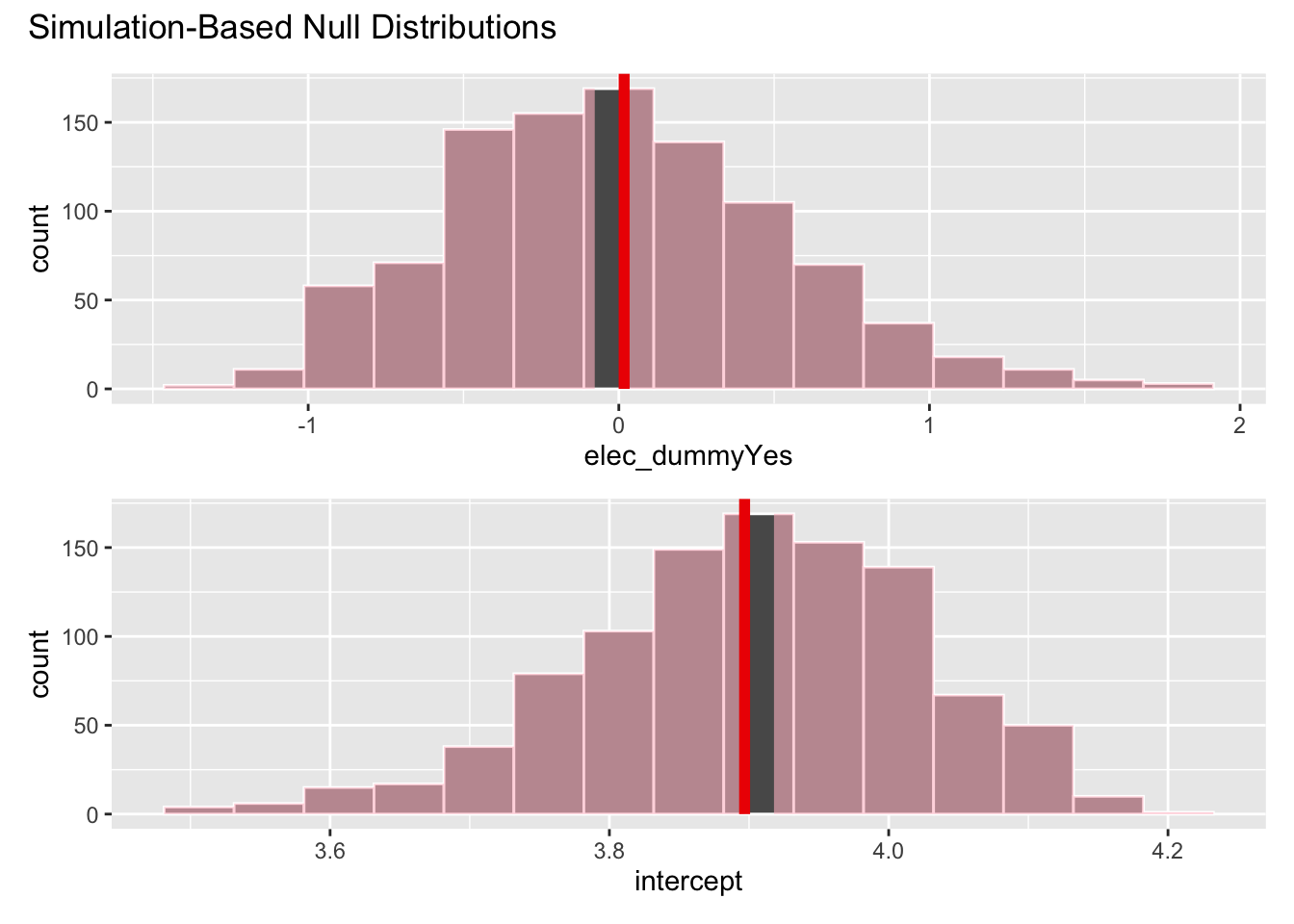
get_p_value(null_dist, obs_fit, direction = "both")# A tibble: 2 × 2
term p_value
<chr> <dbl>
1 elec_dummyYes 0.928
2 intercept 0.928When we checked the linearity assumptions for this model, we discovered some problems.
Recall the technical conditions for linear regression:
- L: linear model
- I: independent observations
- N: points are normally distributed around the line
- E: equal variability around the line for all values of the explanatory variable
# augment() allows us to extract observation-level statistics from a model object
fines_elec_dummy_aug <- augment(fines_elec_dummy_fit, new_data = traffic_fines)
fines_elec_dummy_aug
# A tibble: 1,025 × 97
.pred .resid year county_code county_name vehicle_code_fines
<dbl> <dbl> <dbl> <dbl> <chr> <dbl>
1 3.90 -0.507 2003 1 Alameda 4973766
2 3.90 -0.107 2004 1 Alameda 5701454
3 3.90 -0.899 2005 1 Alameda 4645572
4 3.91 -0.639 2006 1 Alameda 5256212
5 3.90 -0.591 2007 1 Alameda 5498544
6 3.90 -0.388 2008 1 Alameda 6124421
7 3.90 -0.276 2009 1 Alameda 6346925
8 3.91 -0.713 2010 1 Alameda 5753802
9 3.90 -1.15 2011 1 Alameda 5154709
10 3.90 -1.63 2012 1 Alameda 4409751
# ℹ 1,015 more rows
# ℹ 91 more variables: vehicle_code_fines_i_p <dbl>, elec_dummy <chr>,
# sheriff_incumb <dbl>, pre_elec <dbl>, no_incumb <dbl>, incumb <dbl>,
# sheriff_margin <dbl>, rep_share <dbl>, dem_share <dbl>,
# otherparty_share <dbl>, white_share <dbl>, asian_share <dbl>,
# black_share <dbl>, hispanic_share <dbl>, other_share <dbl>,
# young_drivers <dbl>, density <dbl>, areain_square_miles <dbl>, …# the linear regression model
ggplot(
data = fines_elec_dummy_aug,
mapping = aes(
x = as.numeric(elec_dummy == "Yes"),
y = vehicle_code_fines_i_p
)
) +
geom_point() +
geom_smooth(method = "lm")`geom_smooth()` using formula = 'y ~ x'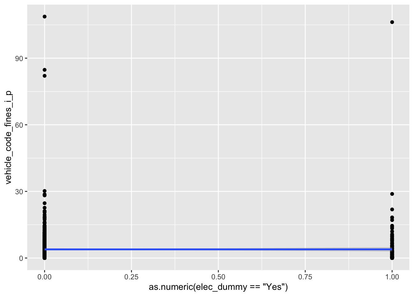
# distribution of the residuals
ggplot(data = fines_elec_dummy_aug, mapping = aes(x = .resid)) +
  geom_histogram()
`stat_bin()` using `bins = 30`. Pick better value `binwidth`.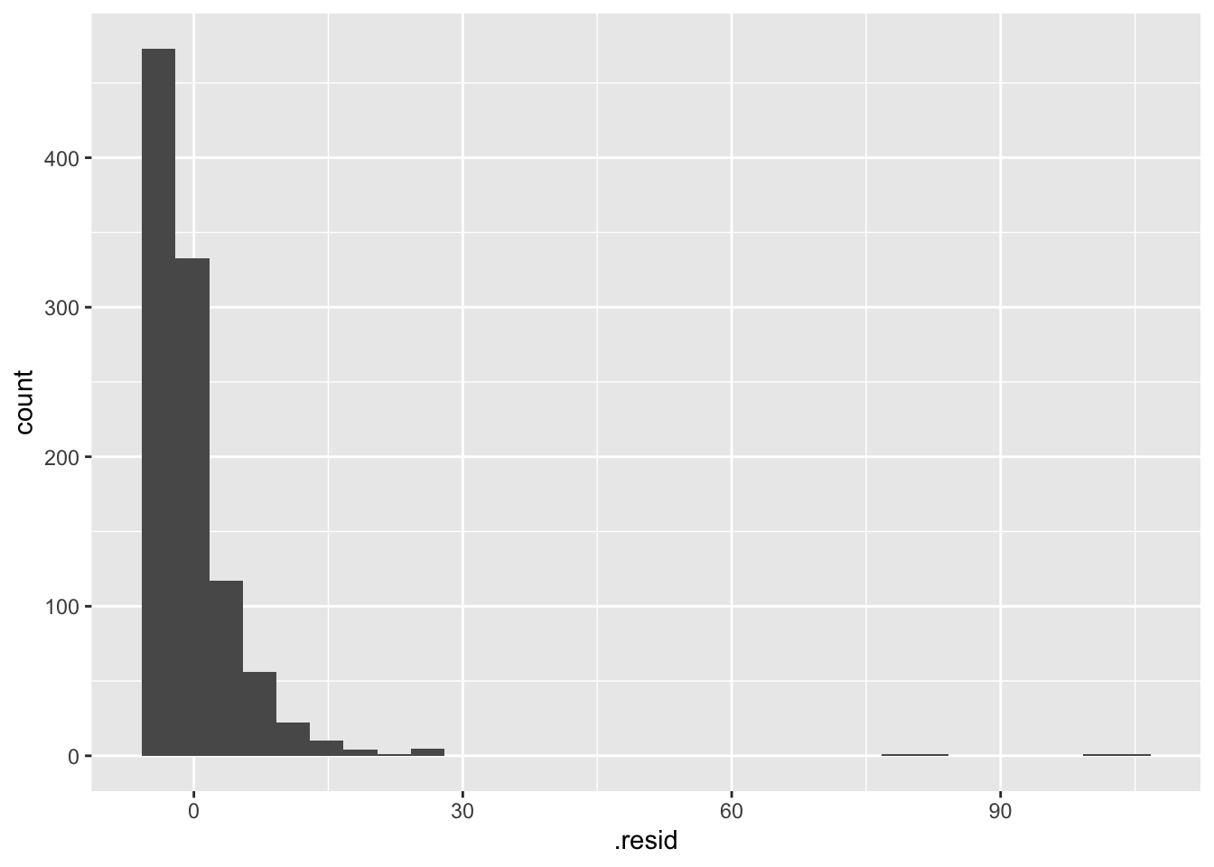
# use the .resid column to plot the predicted values vs. the residuals
# jitter because the explanatory variable only has 2 unique values
ggplot(data = fines_elec_dummy_aug, mapping = aes(x = .pred, y = .resid)) +
  geom_jitter() +
  geom_hline(yintercept = 0, linetype = "dashed")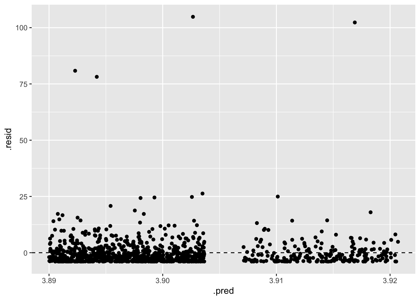
-
L: linear model
Doesn’t seem very linear in the relationship. The fact that we have a categorical variable as the predictor is not inherently a problem, but it doesn’t seem like there is a straight, monotonic relationship between the predictor and the response.
-
I: independent observations
Absolutely no. There are many reasons why the observations are not independent. The obvious reason is that it is a time series cross-sectional (TSCS) panel structure. Each county is observed over multiple years, and the observations within a county are likely to be correlated. Alternatively, each year is observed over multiple counties, and the observations within a year are likely to be correlated.
-
N: points are normally distributed around the line
No. The boxplot earlier shows there are many outliers in the data. The residuals are not normally distributed around the line.
-
E: equal variability around the line for all values of the explanatory variable
No. The residuals are not equally variable around the line for all values of the explanatory variable. The residuals are more variable for counties in an election year than for counties not in an election year.
Today we will build a series of more robust models to better evaluate the hypotheses.
Estimate a multiple variables model
One possible problem with our model yesterday was omitted variable bias. Perhaps we omitted a crucial variable that explains the differences in per capita traffic fine revenue. Since median household income seemed to be predictive of the outcome, let’s estimate a model that includes both whether or not it is an election year and median household income.
Demo: Estimate a model that includes both elec_dummy and med_inc.
fines_inc_elec_fit <- linear_reg() |>
  fit(vehicle_code_fines_i_p ~ med_inc + elec_dummy, data = traffic_fines)

tidy(fines_inc_elec_fit)
# A tibble: 3 × 5
term estimate std.error statistic p.value
<chr> <dbl> <dbl> <dbl> <dbl>
1 (Intercept) 6.93 0.770 8.99 1.16e-18
2 med_inc -0.0000546 0.0000131 -4.17 3.37e- 5
3 elec_dummyYes 0.0400 0.539 0.0743 9.41e- 1Your turn: Interpret the coefficients of the model above.
-
Intercept: Add response here.
Counties not in an election year and with median household income of $0 are expected to earn, on average, $6.93 per capita in traffic fines revenue.
-
Coefficient for median household income:
All else held constant, for each $1,000 increase in median household income, per capita traffic fines revenue is expected to decrease by $0.055.
-
Coefficient for whether or not it is an election year:
All else held constant, counties in an election year are expected to earn, on average, $0.04 more per capita in traffic fines revenue than counties not in an election year.
Hypothesis test
Demo: Use permutation-based methods to conduct the hypothesis test.
-
Median household income
-
Null hypothesis: There is no linear relationship between median household income and per capita traffic fines revenue.
\[H_0: \beta_1 = 0\]
-
Alternative hypothesis: There is some linear relationship between median household income and per capita traffic fines revenue.
\[H_A: \beta_1 \neq 0\]
-
-
Whether or not it is an election year
-
Null hypothesis: There is no linear relationship between whether or not it is an election year and per capita traffic fines revenue.
\[H_0: \beta_2 = 0\]
-
Alternative hypothesis: There is some linear relationship between whether or not it is an election year and per capita traffic fines revenue.
\[H_A: \beta_2 \neq 0\]
-
# calculate observed fit
obs_fit <- traffic_fines |>
  specify(vehicle_code_fines_i_p ~ med_inc + elec_dummy) |>
  fit()

# generate permuted null distribution
null_dist <- traffic_fines |>
  specify(vehicle_code_fines_i_p ~ med_inc + elec_dummy) |>
  hypothesize(null = "independence") |>
  generate(reps = 1000, type = "permute") |>
  fit()

# visualize and calculate p-value
visualize(null_dist) +
  shade_p_value(obs_fit, direction = "both")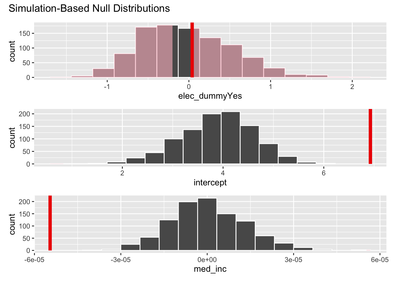
get_p_value(null_dist, obs_fit, direction = "both")Warning: Please be cautious in reporting a p-value of 0. This result is an approximation
based on the number of `reps` chosen in the `generate()` step.
ℹ See `get_p_value()` (`?infer::get_p_value()`) for more information.
Please be cautious in reporting a p-value of 0. This result is an approximation
based on the number of `reps` chosen in the `generate()` step.
ℹ See `get_p_value()` (`?infer::get_p_value()`) for more information.# A tibble: 3 × 2
term p_value
<chr> <dbl>
1 elec_dummyYes 0.842
2 intercept 0
3 med_inc 0 Your turn: Interpret the results of the hypothesis test. Use a significance level of 5%.
- With respect to median household income, the probability of observing a relationship as strong as the one in the data if the null hypothesis is true is less than \(0.001\). Since this is less than 0.05, we reject the null hypothesis and conclude that there is a relationship between median household income and per capita traffic fines revenue.
- With respect to whether or not it is an election year, the probability of observing a relationship as strong as the one in the data if the null hypothesis is true is \(0.842\). Since this is greater than 0.05, we fail to reject the null hypothesis and cannot conclude that there is a relationship between whether or not it is an election year and per capita traffic fines revenue.
Transform a variable
Let’s examine the per capita traffic fines revenue.
Your turn: Run the code chunk below and create two separate plots. How are the two plots different than each other? Which plot’s better depicts an unskewed variable?
# Plot A
ggplot(
  data = traffic_fines,
  mapping = aes(x = vehicle_code_fines_i_p)
) +
  geom_histogram()
`stat_bin()` using `bins = 30`. Pick better value `binwidth`.# Plot B
ggplot(
data = traffic_fines,
mapping = aes(x = vehicle_code_fines_i_p)
) +
geom_histogram() +
scale_x_log10()Warning in scale_x_log10(): log-10 transformation introduced infinite values.`stat_bin()` using `bins = 30`. Pick better value `binwidth`.Warning: Removed 87 rows containing non-finite outside the scale range
(`stat_bin()`).![]()
![]()
Fit the model
Demo: Fit a linear regression model with the transformed outcome variable.
# calculate natural-log transformed outcome
traffic_fines <- traffic_fines |>
  mutate(
    log_vehicle_code_fines_i_p = log(vehicle_code_fines_i_p),
    # replace -Inf with NA - these were counties with $0 in traffic fine revenue
    log_vehicle_code_fines_i_p = if_else(
      log_vehicle_code_fines_i_p == -Inf,
      NA,
      log_vehicle_code_fines_i_p
    )
  )

fines_elec_log_fit <- linear_reg() |>
  fit(log_vehicle_code_fines_i_p ~ elec_dummy, data = traffic_fines)

tidy(fines_elec_log_fit)
# A tibble: 2 × 5
term estimate std.error statistic p.value
<chr> <dbl> <dbl> <dbl> <dbl>
1 (Intercept) 0.544 0.0657 8.28 4.34e-16
2 elec_dummyYes -0.117 0.139 -0.845 3.98e- 1Your turn: Interpret the coefficients of the model above.
Intercept: Counties not in an election year are expected to earn, on average, \(e^{0\\.544} \approx \$1\\.72\) per capita in traffic fines revenue.
Slope: Counties in an election year are expected to earn, on average, \(100 \times [e^{−0\\.117} - 1] \approx 11\\.05%\)% less per capita in traffic fines revenue than those not in an election year.
Conduct a hypothesis test
Demo: Use permutation-based methods to conduct the hypothesis test.
# calculate observed fit
obs_fit <- traffic_fines |>
  specify(log_vehicle_code_fines_i_p ~ elec_dummy) |>
  fit()
Warning: Removed 87 rows containing missing values.# generate permuted null distribution
null_dist <- traffic_fines |>
specify(log_vehicle_code_fines_i_p ~ elec_dummy) |>
hypothesize(null = "independence") |>
generate(reps = 1000, type = "permute") |>
fit()Warning: Removed 87 rows containing missing values.# visualize and calculate p-value
visualize(null_dist) +
shade_p_value(obs_fit, direction = "both")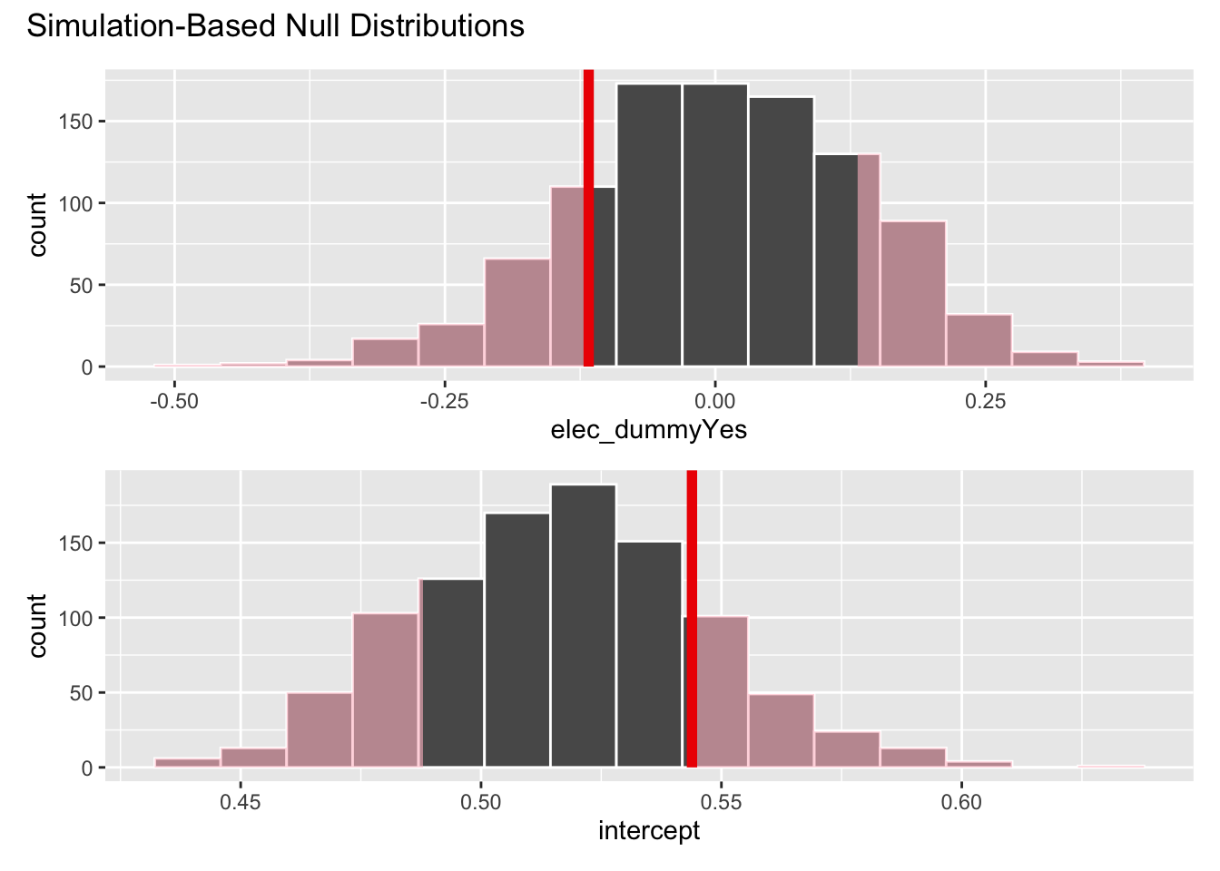
get_p_value(null_dist, obs_fit, direction = "both")# A tibble: 2 × 2
term p_value
<chr> <dbl>
1 elec_dummyYes 0.35
2 intercept 0.35Your turn: Interpret the \(p\)-value in context of the data and the research question. Use a significance level of 5%.
If in fact the true relationship between whether or not it is an election and per capita traffic fines revenue is zero, the probability of observing a relationship as strong as the one in the data is \(0.35\). Since this is greater than 0.05, we fail to reject the null hypothesis and cannot conclude that there is a relationship between whether or not it is an election and per capita traffic fines revenue.
What about other differences?
So far we have only estimated a model with at most two explanatory variables. Yet there are many other variables in the data set that could explain the variation in per capita traffic fines revenue.
Recall that the data set is a panel structure - we observe multiple counties over multiple years. This violates the linear model assumption of independence of the observations. Consider the most obvious example - traffic fines revenue within a single county is likely to be correlated across years (e.g. knowing how much revenue was generated in Los Angeles County this year allows me to make a better guess for next year’s revenue).
Fixed effects
One way we can account for this by estimating a fixed effects model. This model includes a separate coefficient for each county, which allows us to account for the correlation in the data.
Demo: Let’s estimate a model that includes elec_dummy and a fixed effect for each county. We’ll also use the log-transformed outcome of interest.
fines_fe_fit <- linear_reg() |>
  fit(
    log_vehicle_code_fines_i_p ~ elec_dummy + factor(county_name),
    data = traffic_fines
  )

tidy(fines_fe_fit)
# A tibble: 57 × 5
term estimate std.error statistic p.value
<chr> <dbl> <dbl> <dbl> <dbl>
1 (Intercept) 0.963 0.214 4.50 7.65e- 6
2 elec_dummyYes -0.0981 0.0708 -1.38 1.67e- 1
3 factor(county_name)Alpine 1.07 0.385 2.77 5.69e- 3
4 factor(county_name)Amador -1.11 0.323 -3.44 6.03e- 4
5 factor(county_name)Butte -0.832 0.458 -1.82 6.95e- 2
6 factor(county_name)Calaveras 0.402 0.302 1.33 1.84e- 1
7 factor(county_name)Colusa 0.0297 0.302 0.0984 9.22e- 1
8 factor(county_name)Contra Costa -0.471 0.302 -1.56 1.19e- 1
9 factor(county_name)Del Norte -5.36 0.370 -14.5 7.97e-43
10 factor(county_name)El Dorado -0.177 0.302 -0.585 5.58e- 1
# ℹ 47 more rowsYour turn: Interpret the coefficient for elec_dummy.
Holding county constant, counties in an election year are expected to earn, on average, \(100 \times [e^{−0\\.098} - 1] \approx 9\\.34%\)% less per capita in traffic fines revenue than those not in an election year.
Conduct a hypothesis test
Demo: Use permutation-based methods to conduct the hypothesis test.
# calculate observed fit
obs_fit <- traffic_fines |>
  specify(log_vehicle_code_fines_i_p ~ elec_dummy + factor(county_name)) |>
  fit()
Warning: Removed 87 rows containing missing values.# generate permuted null distribution
null_dist <- traffic_fines |>
specify(log_vehicle_code_fines_i_p ~ elec_dummy + factor(county_name)) |>
hypothesize(null = "independence") |>
generate(reps = 1000, type = "permute") |>
fit()Warning: Removed 87 rows containing missing values.# calculate p-value
get_p_value(null_dist, obs_fit, direction = "both")Warning: Please be cautious in reporting a p-value of 0. This result is an approximation
based on the number of `reps` chosen in the `generate()` step.
ℹ See `get_p_value()` (`?infer::get_p_value()`) for more information.Warning: Please be cautious in reporting a p-value of 0. This result is an approximation
based on the number of `reps` chosen in the `generate()` step.
ℹ See `get_p_value()` (`?infer::get_p_value()`) for more information.
Please be cautious in reporting a p-value of 0. This result is an approximation
based on the number of `reps` chosen in the `generate()` step.
ℹ See `get_p_value()` (`?infer::get_p_value()`) for more information.
Please be cautious in reporting a p-value of 0. This result is an approximation
based on the number of `reps` chosen in the `generate()` step.
ℹ See `get_p_value()` (`?infer::get_p_value()`) for more information.
Please be cautious in reporting a p-value of 0. This result is an approximation
based on the number of `reps` chosen in the `generate()` step.
ℹ See `get_p_value()` (`?infer::get_p_value()`) for more information.
Please be cautious in reporting a p-value of 0. This result is an approximation
based on the number of `reps` chosen in the `generate()` step.
ℹ See `get_p_value()` (`?infer::get_p_value()`) for more information.
Please be cautious in reporting a p-value of 0. This result is an approximation
based on the number of `reps` chosen in the `generate()` step.
ℹ See `get_p_value()` (`?infer::get_p_value()`) for more information.
Please be cautious in reporting a p-value of 0. This result is an approximation
based on the number of `reps` chosen in the `generate()` step.
ℹ See `get_p_value()` (`?infer::get_p_value()`) for more information.# A tibble: 57 × 2
term p_value
<chr> <dbl>
1 elec_dummyYes 0.476
2 factor(county_name)Alpine 0.158
3 factor(county_name)Amador 0.072
4 factor(county_name)Butte 0.298
5 factor(county_name)Calaveras 0.496
6 factor(county_name)Colusa 0.944
7 factor(county_name)Contra Costa 0.402
8 factor(county_name)Del Norte 0
9 factor(county_name)El Dorado 0.756
10 factor(county_name)Fresno 0.762
# ℹ 47 more rowsYour turn: Interpret the results of the hypothesis test in context of the data and the research question. Use a significance level of 5%.
If in fact the true relationship between whether or not it is an election and per capita traffic fines revenue is zero, the probability of observing a relationship as strong as the one in the data is \(0.476\). Since this is greater than 0.05, we fail to reject the null hypothesis and cannot conclude that there is a relationship between whether or not it is an election and per capita traffic fines revenue.
Include everything
Finally, let’s estimate a model that includes all the variables in the data set.
# keep all variables used in original analysis - table 1 column 2
tf_replication <- traffic_fines |>
  select(
    log_vehicle_code_fines_i_p,
    elec_dummy,
    dem_share,
    otherparty_share,
    asian_share,
    black_share,
    hispanic_share,
    other_share,
    young_drivers,
    density,
    med_inc,
    unemp,
    own_source_share,
    emp_goods,
    emp_service,
    pay_goods_i,
    pay_service_i,
    arte_share,
    collect_share,
    cnty_le_sworn_1000p,
    felony_tot_1000p,
    misdemeanor_tot_1000p,
    county_name,
    # separate columns for each county to include the year trend
    starts_with("i_trend")
  )

fines_all_fit <- linear_reg() |>
  # use all remaining columns as predictors
  fit(log_vehicle_code_fines_i_p ~ ., data = tf_replication)

tidy(fines_all_fit)
# A tibble: 134 × 5
term estimate std.error statistic p.value
<chr> <dbl> <dbl> <dbl> <dbl>
1 (Intercept) 3.13 10.7 0.294 0.769
2 elec_dummyYes -0.0895 0.0505 -1.77 0.0767
3 dem_share -0.0275 0.0128 -2.14 0.0327
4 otherparty_share -0.0285 0.0165 -1.73 0.0836
5 asian_share -0.0298 0.182 -0.164 0.870
6 black_share -1.05 0.346 -3.03 0.00252
7 hispanic_share 0.450 0.0795 5.66 0.0000000215
8 other_share 1.30 0.414 3.14 0.00175
9 young_drivers 0.124 0.0620 2.00 0.0459
10 density 0.000306 0.00448 0.0683 0.946
# ℹ 124 more rowsYour turn: Interpret the coefficient for elec_dummy.
Holding all other variables constant, counties in an election year are expected to earn, on average, \(100 \times [e^{−0\\.089} - 1] \approx 8\\.56%\)% less per capita in traffic fines revenue than those not in an election year.
Conduct a hypothesis test
At this point it seems reasonable that we have met the assumptions of the linear model. Let’s conduct a hypothesis test to evaluate the relationship between whether or not it is an election year and per capita traffic fines revenue. Instead of relying on the permutation-based approach, we will use the standard \(t\)-test that was reported when we estimated the model above.
Your turn: Interpret the results of the hypothesis test in context of the data and the research question. Use a significance level of 5%.
If in fact the true relationship between whether or not it is an election and per capita traffic fines revenue is zero, the probability of observing a relationship as strong as the one in the data is \(0.0767\). Since this is greater than 0.05, we fail to reject the null hypothesis and cannot conclude that there is a relationship between whether or not it is an election and per capita traffic fines revenue.
Comparing across models
Let’s compare the models we estimated today. Remember that we are interested in the model simplest best model.
glance(fines_elec_dummy_fit)# A tibble: 1 × 12
r.squared adj.r.squared sigma statistic p.value df logLik AIC BIC
<dbl> <dbl> <dbl> <dbl> <dbl> <dbl> <dbl> <dbl> <dbl>
1 0.000000968 -0.000977 7.23 0.000990 0.975 1 -3481. 6969. 6983.
# ℹ 3 more variables: deviance <dbl>, df.residual <int>, nobs <int>glance(fines_inc_elec_fit)# A tibble: 1 × 12
r.squared adj.r.squared sigma statistic p.value df logLik AIC BIC
<dbl> <dbl> <dbl> <dbl> <dbl> <dbl> <dbl> <dbl> <dbl>
1 0.0167 0.0148 7.17 8.67 0.000184 2 -3473. 6953. 6973.
# ℹ 3 more variables: deviance <dbl>, df.residual <int>, nobs <int>glance(fines_elec_log_fit)# A tibble: 1 × 12
r.squared adj.r.squared sigma statistic p.value df logLik AIC BIC
<dbl> <dbl> <dbl> <dbl> <dbl> <dbl> <dbl> <dbl> <dbl>
1 0.000763 -0.000305 1.77 0.715 0.398 1 -1867. 3739. 3754.
# ℹ 3 more variables: deviance <dbl>, df.residual <int>, nobs <int>glance(fines_fe_fit)# A tibble: 1 × 12
r.squared adj.r.squared sigma statistic p.value df logLik AIC BIC
<dbl> <dbl> <dbl> <dbl> <dbl> <dbl> <dbl> <dbl> <dbl>
1 0.754 0.739 0.906 48.3 7.62e-229 56 -1209. 2533. 2814.
# ℹ 3 more variables: deviance <dbl>, df.residual <int>, nobs <int>glance(fines_all_fit)# A tibble: 1 × 12
r.squared adj.r.squared sigma statistic p.value df logLik AIC BIC
<dbl> <dbl> <dbl> <dbl> <dbl> <dbl> <dbl> <dbl> <dbl>
1 0.896 0.878 0.610 49.5 4.38e-297 132 -750. 1769. 2411.
# ℹ 3 more variables: deviance <dbl>, df.residual <int>, nobs <int>Your turn: Which model do you believe is most appropriate? Why?
The model that includes all variables is the most appropriate. The fixed-effects model is potentially a good choice with a high adjusted-\(R^2\) value, but the model that also includes the control variables has an adjusted-\(R^2\) value nearly 14 points higher. In this situation, the additional complexity of the model is outweighed by the improvement in performance.
sessioninfo::session_info()─ Session info ───────────────────────────────────────────────────────────────
setting value
version R version 4.5.2 (2025-10-31)
os macOS Tahoe 26.4
system aarch64, darwin20
ui X11
language (EN)
collate en_US.UTF-8
ctype en_US.UTF-8
tz America/New_York
date 2026-04-02
pandoc 3.4 @ /usr/local/bin/ (via rmarkdown)
quarto 1.9.36 @ /usr/local/bin/quarto
─ Packages ───────────────────────────────────────────────────────────────────
! package * version date (UTC) lib source
P archive 1.1.12.1 2025-12-24 [?] RSPM
P backports 1.5.0 2024-05-23 [?] RSPM (R 4.5.0)
P base64enc 0.1-3 2015-07-28 [?] RSPM (R 4.5.0)
P bit 4.6.0 2025-03-06 [?] RSPM (R 4.5.0)
P bit64 4.6.0-1 2025-01-16 [?] RSPM (R 4.5.0)
P broom * 1.0.11 2025-12-04 [?] RSPM (R 4.5.0)
P class 7.3-23 2025-01-01 [?] RSPM (R 4.5.0)
P cli 3.6.5 2025-04-23 [?] RSPM (R 4.5.0)
P codetools 0.2-20 2024-03-31 [?] RSPM (R 4.5.0)
P crayon 1.5.3 2024-06-20 [?] RSPM (R 4.5.0)
P data.table 1.18.0 2025-12-24 [?] RSPM (R 4.5.0)
P dials * 1.4.2 2025-09-04 [?] RSPM
P DiceDesign 1.10 2023-12-07 [?] RSPM (R 4.5.0)
P digest 0.6.39 2025-11-19 [?] RSPM (R 4.5.0)
P dplyr * 1.2.0 2026-02-03 [?] RSPM
P evaluate 1.0.5 2025-08-27 [?] RSPM (R 4.5.0)
P farver 2.1.2 2024-05-13 [?] RSPM (R 4.5.0)
P fastmap 1.2.0 2024-05-15 [?] RSPM (R 4.5.0)
P forcats * 1.0.1 2025-09-25 [?] RSPM (R 4.5.0)
P furrr 0.3.1 2022-08-15 [?] RSPM
P future 1.68.0 2025-11-17 [?] RSPM
P future.apply 1.20.1 2025-12-09 [?] CRAN (R 4.5.2)
P generics 0.1.4 2025-05-09 [?] RSPM (R 4.5.0)
P ggplot2 * 4.0.1 2025-11-14 [?] RSPM (R 4.5.0)
P globals 0.18.0 2025-05-08 [?] RSPM
P glue 1.8.0 2024-09-30 [?] RSPM (R 4.5.0)
P gower 1.0.2 2024-12-17 [?] RSPM
P GPfit 1.0-9 2025-04-12 [?] RSPM (R 4.5.0)
P gtable 0.3.6 2024-10-25 [?] RSPM (R 4.5.0)
P hardhat 1.4.2 2025-08-20 [?] RSPM
P here 1.0.2 2025-09-15 [?] CRAN (R 4.5.0)
P hms 1.1.4 2025-10-17 [?] RSPM (R 4.5.0)
P htmltools 0.5.9 2025-12-04 [?] RSPM (R 4.5.0)
P htmlwidgets 1.6.4 2023-12-06 [?] RSPM (R 4.5.0)
P infer * 1.1.0 2025-12-18 [?] CRAN (R 4.5.2)
P ipred 0.9-15 2024-07-18 [?] RSPM
P jsonlite 2.0.0 2025-03-27 [?] RSPM (R 4.5.0)
P knitr 1.51 2025-12-20 [?] RSPM (R 4.5.0)
P labeling 0.4.3 2023-08-29 [?] RSPM (R 4.5.0)
P lattice 0.22-7 2025-04-02 [?] RSPM (R 4.5.0)
P lava 1.8.2 2025-10-30 [?] RSPM
P lhs 1.2.0 2024-06-30 [?] RSPM (R 4.5.0)
P lifecycle 1.0.5 2026-01-08 [?] RSPM (R 4.5.0)
P listenv 0.10.0 2025-11-02 [?] RSPM
P lubridate * 1.9.4 2024-12-08 [?] RSPM (R 4.5.0)
P magrittr 2.0.4 2025-09-12 [?] RSPM (R 4.5.0)
P MASS 7.3-65 2025-02-28 [?] RSPM (R 4.5.0)
P Matrix 1.7-4 2025-08-28 [?] RSPM (R 4.5.0)
P mgcv 1.9-4 2025-11-07 [?] CRAN (R 4.5.0)
P modeldata * 1.5.1 2025-08-22 [?] RSPM
P nlme 3.1-168 2025-03-31 [?] RSPM (R 4.5.0)
P nnet 7.3-20 2025-01-01 [?] RSPM (R 4.5.0)
P otel 0.2.0 2025-08-29 [?] RSPM (R 4.5.0)
P parallelly 1.46.0 2025-12-12 [?] CRAN (R 4.5.2)
P parsnip * 1.4.0 2025-12-01 [?] CRAN (R 4.5.2)
P patchwork 1.3.2 2025-08-25 [?] RSPM
P pillar 1.11.1 2025-09-17 [?] RSPM (R 4.5.0)
P pkgconfig 2.0.3 2019-09-22 [?] RSPM (R 4.5.0)
P prodlim 2025.04.28 2025-04-28 [?] RSPM
P purrr * 1.2.0 2025-11-04 [?] CRAN (R 4.5.0)
P R6 2.6.1 2025-02-15 [?] RSPM (R 4.5.0)
P RColorBrewer 1.1-3 2022-04-03 [?] RSPM (R 4.5.0)
P Rcpp 1.1.0 2025-07-02 [?] RSPM (R 4.5.0)
P readr * 2.1.6 2025-11-14 [?] RSPM (R 4.5.0)
P recipes * 1.3.1 2025-05-21 [?] RSPM
renv 1.1.5 2025-07-24 [1] RSPM (R 4.5.0)
P repr 1.1.7 2024-03-22 [?] RSPM
P rlang 1.1.7 2026-01-09 [?] RSPM (R 4.5.0)
P rmarkdown 2.30 2025-09-28 [?] RSPM (R 4.5.0)
P rpart 4.1.24 2025-01-07 [?] RSPM (R 4.5.0)
P rprojroot 2.1.1 2025-08-26 [?] RSPM (R 4.5.0)
P rsample * 1.3.1 2025-07-29 [?] RSPM
P rstudioapi 0.17.1 2024-10-22 [?] RSPM (R 4.5.0)
P S7 0.2.1 2025-11-14 [?] RSPM (R 4.5.0)
P scales * 1.4.0 2025-04-24 [?] RSPM (R 4.5.0)
P sessioninfo 1.2.3 2025-02-05 [?] RSPM (R 4.5.0)
P skimr * 2.2.1 2025-07-26 [?] RSPM
P sparsevctrs 0.3.5 2025-12-09 [?] CRAN (R 4.5.2)
P stringi 1.8.7 2025-03-27 [?] RSPM (R 4.5.0)
P stringr * 1.6.0 2025-11-04 [?] RSPM (R 4.5.0)
P survival 3.8-3 2024-12-17 [?] RSPM (R 4.5.0)
P tailor * 0.1.0 2025-08-25 [?] RSPM
P tibble * 3.3.0 2025-06-08 [?] RSPM (R 4.5.0)
P tidymodels * 1.4.1 2025-09-08 [?] RSPM
P tidyr * 1.3.2 2025-12-19 [?] RSPM (R 4.5.0)
P tidyselect 1.2.1 2024-03-11 [?] RSPM (R 4.5.0)
P tidyverse * 2.0.0 2023-02-22 [?] RSPM (R 4.5.0)
P timechange 0.3.0 2024-01-18 [?] RSPM (R 4.5.0)
P timeDate 4051.111 2025-10-17 [?] RSPM
P tune * 2.0.1 2025-10-17 [?] RSPM
P tzdb 0.5.0 2025-03-15 [?] RSPM (R 4.5.0)
P utf8 1.2.6 2025-06-08 [?] RSPM (R 4.5.0)
P vctrs 0.7.1 2026-01-23 [?] RSPM
P vroom 1.6.7 2025-11-28 [?] RSPM (R 4.5.0)
P withr 3.0.2 2024-10-28 [?] RSPM (R 4.5.0)
P workflows * 1.3.0 2025-08-27 [?] RSPM
P workflowsets * 1.1.1 2025-05-27 [?] RSPM
P xfun 0.55 2025-12-16 [?] CRAN (R 4.5.2)
P yaml 2.3.12 2025-12-10 [?] RSPM (R 4.5.0)
P yardstick * 1.3.2 2025-01-22 [?] RSPM
[1] /Users/bcs88/Projects/info-2950/course-site/renv/library/macos/R-4.5/aarch64-apple-darwin20
[2] /Users/bcs88/Library/Caches/org.R-project.R/R/renv/sandbox/macos/R-4.5/aarch64-apple-darwin20/4cd76b74
* ── Packages attached to the search path.
P ── Loaded and on-disk path mismatch.
──────────────────────────────────────────────────────────────────────────────Footnotes
The codebook is available from Dataverse. The data set has been lightly cleaned for the application exercise.↩︎