HW 06 - Evaluating claims from astrology

Homework

Modified

March 19, 2026

Important

This homework is due March 26 at 11:59pm.

Learning objectives

Construct confidence intervals
Conduct hypothesis tests
Interpret confidence intervals and results of hypothesis tests in context of the data

Getting started

Go to the info2951-sp26 organization on GitHub. Click on the repo with the prefix hw-06. It contains the starter documents you need to complete the homework.
Clone the repo and start a new workspace in Positron. See the Homework 0 instructions for details on cloning a repo and starting a new R project.

General guidance

Guidelines + tips

As we’ve discussed in lecture, your plots should include an informative title, axes should be labeled, and careful consideration should be given to aesthetic choices.

Remember that continuing to develop a sound workflow for reproducible data analysis is important as you complete the homework and other assignments in this course. There will be periodic reminders in this assignment to remind you to render, commit, and push your changes to GitHub. You should have at least 3 commits with meaningful commit messages by the end of the assignment.

Workflow + formatting

Make sure to

Update author name on your document.
Label all code chunks informatively and concisely.
Follow the Tidyverse code style guidelines.
Make at least 3 commits.
Resize figures where needed, avoid tiny or huge plots.
Turn in an organized, well formatted document.

Packages

We’ll use the {tidyverse} package for much of the data wrangling and visualization and the {tidymodels} package for modeling and inference. You can load them by running the following in your Console:

library(tidyverse)
library(tidymodels)

Data

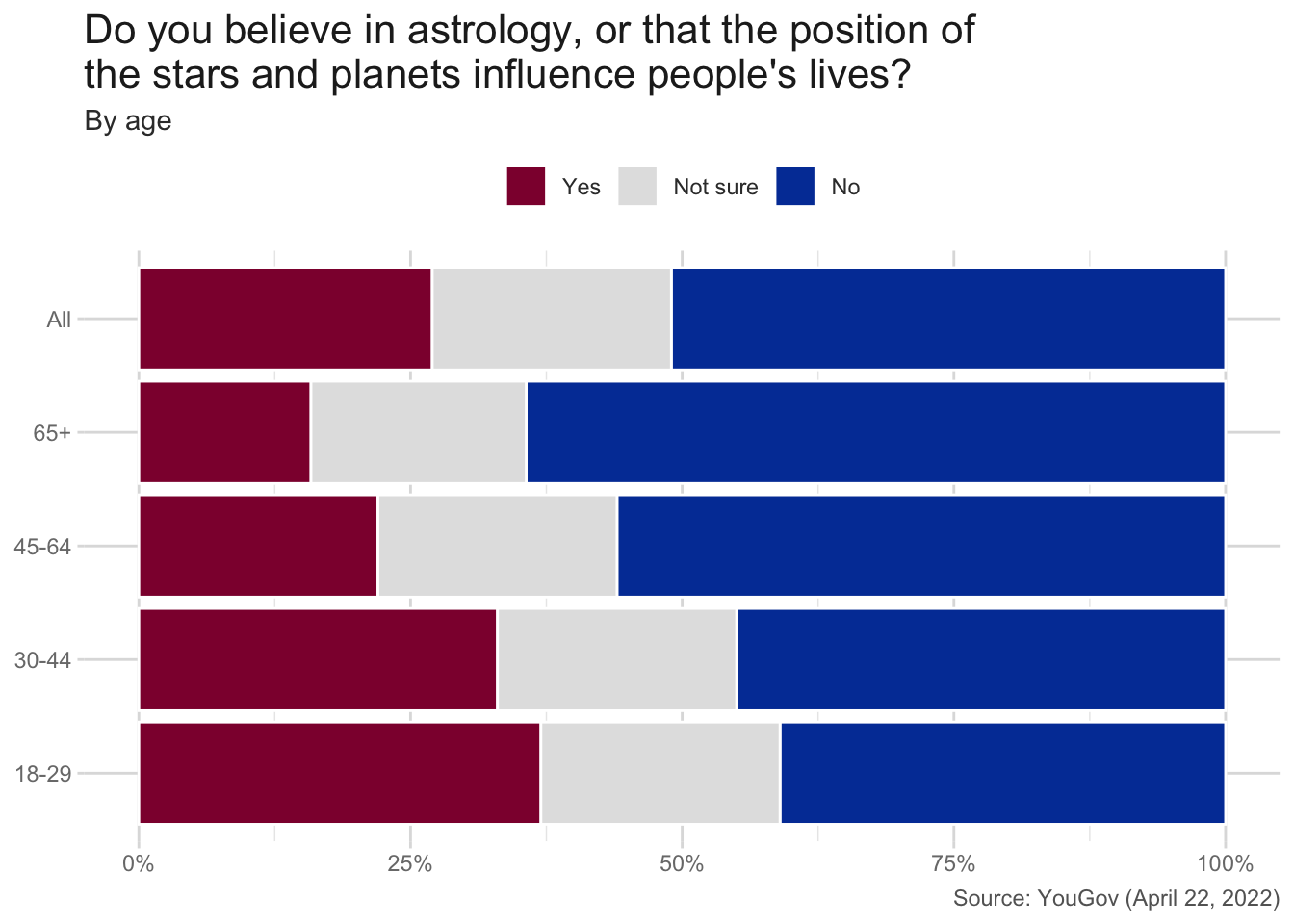
Astrology, or the belief that the position of the stars and planets can affect people’s lives, remains popular with many people in the United States. As of 2022, 27% of Americans believe that the position of the stars and planets influence people’s lives (see Figure 1).

Figure 1: Survey results on belief in astrology, by age group. Source: YouGov (April 22, 2022).

To assess the predictive power of astrology, the Clearer Thinking Team ran a study to determine if astrological sun signs (or zodiac signs) predict facts about people’s lives. Their findings? No. Astrological signs were no better than random chance at predicting people’s behavior and traits.

Some astrologers criticized the study, saying that “of course [they] found that sun signs don’t predict facts about a person’s life, because that’s baby or tabloid astrology. Real astrologers use people’s entire astrological charts to glean insights about them and their lives.”

Given this challenge, Spencer Greenberg and André Ferretti ran a second study to assess whether astrologers could predict people’s zodiac signs (based on astrological charts) given information about individual’s traits and behavior. The authors very kindly published the data from this study, and you will find a cleaned version in data/astrology.csv. The authors originally used traditional hypothesis tests to analyze the data, but given the relatively small sample size you will re-analyze the data using the computational approaches for inference we have learned in this course.

Exercises

Set your random seed

In this homework we’ll be generating random samples. The last thing you want is those samples to change every time you render your document. Be sure to set a fixed seed value in your Quarto document before you perform any randomized tasks.

Exercise 1

Import and review the data. What are the observations in this data set? How many observations are there in our sample? What are the variables? Feel free to consult the original study if you need additional context.

Exercise 2

Can astrologers predict zodiac signs? The original study contains predictions from both individuals with astrological experience and novices. For this exercise, we will focus on the predictions made by individuals with astrological experience (i.e., astrologers).

We want to evaluate the claim that astrologers can predict people’s zodiac signs better than random chance. Since each participant generated 12 predictions (each with 5 possible answers), random chance should result in an average of \(12 / 5 \approx 2.4\) correct predictions out of 12.

\[H_0: \mu = 2.4\]

Our alternative hypothesis should reflect the research question, i.e. astrologers perform better than random guessing. Since the research question states a direction for the change, we can use a one-sided alternative hypothesis:

\[H_A: \mu > 2.4\]

Create a filtered data frame that contains only data from those with astrological experience. Then, calculate the mean number of correct guesses. Run the appropriate hypothesis test, visualize the null distribution, calculate the p-value, and interpret the results in context of the data and the hypothesis test.

Tip

For all hypothesis tests in this homework, use \(\alpha = 0.05\).

Exercise 3

Astrologers and novices. Recall that the original study also collected predictions from novices (i.e., individuals without astrological experience). Consider the relationship between astrological experience and the number of correct predictions. Generate an appropriate plot that displays this relationship, and briefly describe what the plot reveals about the relationship between these two variables.

Exercise 4

Formally test astrologers vs. novices. We can compare the means of the distributions using the following to first group the data by the experience variable, and then calculate the mean correct_answers in these groups using.

astro |>
  group_by(experience) |>
  summarize(
    mean_correct = mean(correct_answers)
  )

# A tibble: 2 × 2
  experience mean_correct
  <chr>             <dbl>
1 Astrologer         2.49
2 Guesser            2.13

There is an observed difference, but is this difference statistically significant? In order to answer this question we will conduct a hypothesis test.

Write the hypotheses for testing if the average number of correct answers from astrologers and novices are different. Run the appropriate hypothesis test, calculate the p-value, and interpret the results in context of the data and the hypothesis test.

Construct a 95% confidence interval for the difference between the average number of correct answers from astrologers and novices. Would you expect the 95% confidence interval to contain 0? Why or why not?

Exercise 5

Assessing substantive significance. Statistical significance does not necessarily imply substantive significance. In the context of this study, a result is substantively significant if astrologers can predict zodiac signs well enough to be practically useful. What would be a substantively significant difference in the average number of correct predictions between astrologers and novices? Justify your answer.

Use this definition of substantive significance along with the results from Exercises 4 to assess whether the difference in average number of correct predictions between astrologers and novices is substantively significant.

Wrap up

Submission

Go to http://www.gradescope.com and click Log in in the top right corner.
Click School Credentials \(\rightarrow\) Cornell University NetID and log in using your NetID credentials.
Click on your INFO 2951 course.
Click on the assignment, and you’ll be prompted to submit it.
Mark all the pages associated with exercise. All the pages of your homework should be associated with at least one question (i.e., should be “checked”).
Select all pages of your .pdf submission to be associated with the “Workflow & formatting” question.

Grading

Component	Points
Ex 1	5
Ex 2	15
Ex 3	5
Ex 4	15
Ex 5	5
Workflow & formatting	5
Total	50

Workflow & formatting criteria

The “Workflow & formatting” component assesses the reproducible workflow. This includes:

At least 3 informative commit messages
Following {tidyverse} code style
All code being visible in rendered PDF without automatic wrapping (no more than 80 characters)
Ensuring reproducibility by setting a random seed value.

Acknowledgments

This assignment is derived from Data Science in a Box and licensed under CC BY-SA 4.0.