AE 15: How much food do you get when you order Chipotle?

Data summary
Name	chipotle
Number of rows	30
Number of columns	7
_______________________
Column type frequency:
character	4
Date	1
numeric	2
________________________
Group variables	None

skim_variable	complete_rate	min	max	n_unique
order	1	6	6	2
meat	1	7	8	2
store	1	7	7	3
food	1	4	7	2

skim_variable	n_missing	complete_rate	min	max	median	n_unique
date	0	1	2024-01-12	2024-02-10	2024-01-26	30

skim_variable	n_missing	complete_rate	mean	sd	p0	p25	p50	p75	p100	hist
day	0	1	15.5	8.80	1.00	8.25	15.50	22.75	30.00	▇▇▇▇▇
weight	0	1	810.8	123.37	510.29	715.82	793.79	907.18	1048.93	▁▆▇▇▂

Typical weight of a Chipotle order

Observed sample

Demo: Visualize the distribution of weight using a histogram and calculate the arithmetic mean.

ggplot(data = chipotle, mapping = aes(x = weight)) +
  geom_histogram()

`stat_bin()` using `bins = 30`. Pick better value with `binw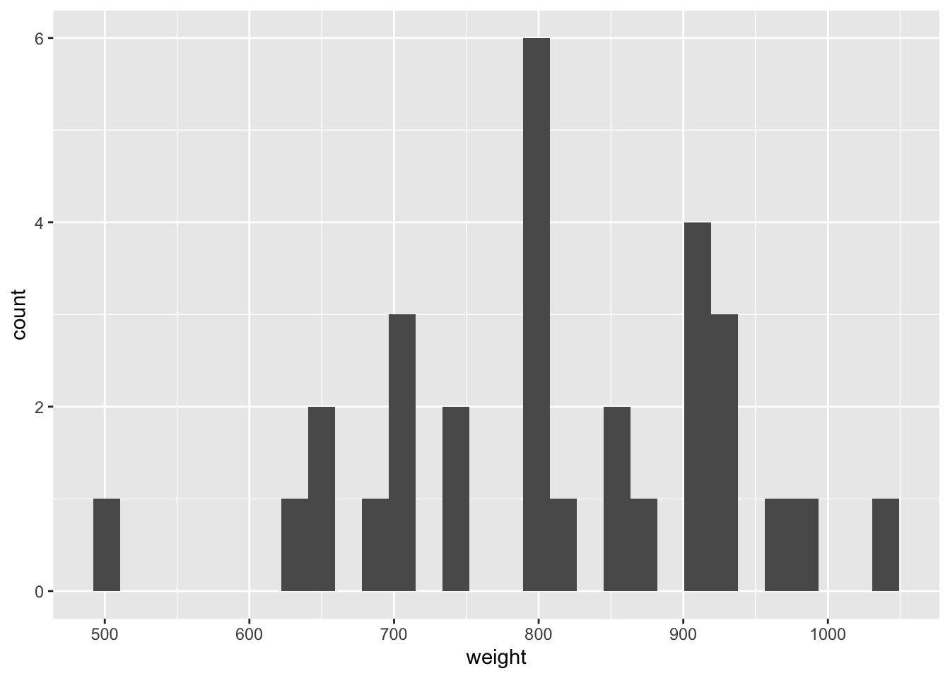idth`.

chipotle |>
  summarize(mean = mean(weight))

# A tibble: 1 × 1
   mean
  <dbl>
1  811.

Your turn:

What is the sample statistic? 810
How large will each bootstrap sample be? 30 observations
How many bootstrap resamples do we need? Enough - usually 1,000 is a good starting point

Generate bootstrap means

Demo: Generate 1,000 bootstrap means of the order weight.

set.seed(123) # to ensure reproducibility

# observed difference
d_hat <- chipotle |>
  specify(response = weight) |>
  calculate(stat = "mean")

boot_df <- chipotle |>
  specify(response = weight) |>
  generate(reps = 1000, type = "bootstrap") |>
  calculate(stat = "mean")

Your turn: Take a glimpse() of boot_df. What do you see?

glimpse(boot_df)

Rows: 1,000
Columns: 2
$ replicate <int> 1, 2, 3, 4, 5, 6, 7, 8, 9, 10, 11, 12, 13, 14, 15, 16, 17, 1…
$ stat      <dbl> 786.2261, 790.0061, 803.2358, 750.3168, 773.9413, 805.1258, …

Your turn: Plot a histogram of boot_df. Where is it centered? Why does this make sense?

visualize(data = boot_df)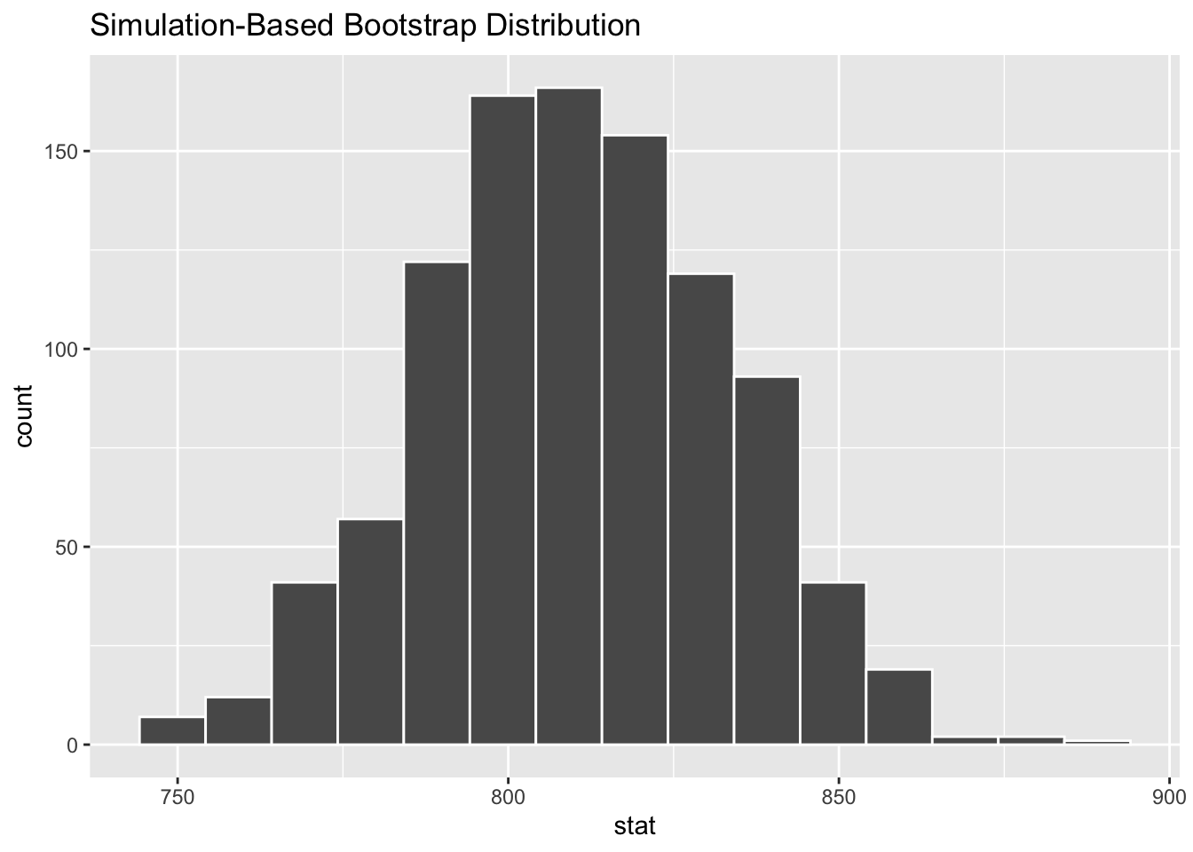

Create a 95% confidence interval

Demo: Now let’s use boot_df to create our 95% confidence interval.

get_ci(x = boot_df, level = 0.95)

# A tibble: 1 × 2
  lower_ci upper_ci
     <dbl>    <dbl>
1     766.     853.

Demo: Let’s visualize our confidence interval by adding a vertical line at each of these values.

visualize(data = boot_df) +
  shade_ci(endpoints = get_ci(x = boot_df, level = 0.95))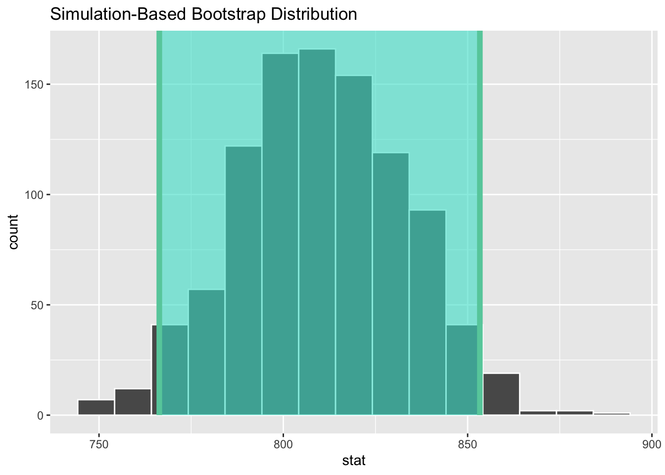

Interpreting confidence intervals

How do we interpret this confidence interval?

There is a 95% probability the true weight of Chipotle orders is between 766 and 854 grams.
There is a 95% probability the weight of Chipotle orders is between 766 and 854 grams.
We are 95% confident the true weight of Chipotle orders is between 766 and 854 grams.
We are 95% confident the weight of Chipotle orders is between 766 and 854 grams.

Alternative confidence intervals

Your turn: Create a 90% confidence interval. Report it below and visualize it with the histogram created above. Is it wider or more narrow than the 95% confidence interval?

get_ci(x = boot_df, level = 0.90)

# A tibble: 1 × 2
  lower_ci upper_ci
     <dbl>    <dbl>
1     772.     846.

visualize(data = boot_df) +
  shade_ci(endpoints = get_ci(x = boot_df, level = 0.90))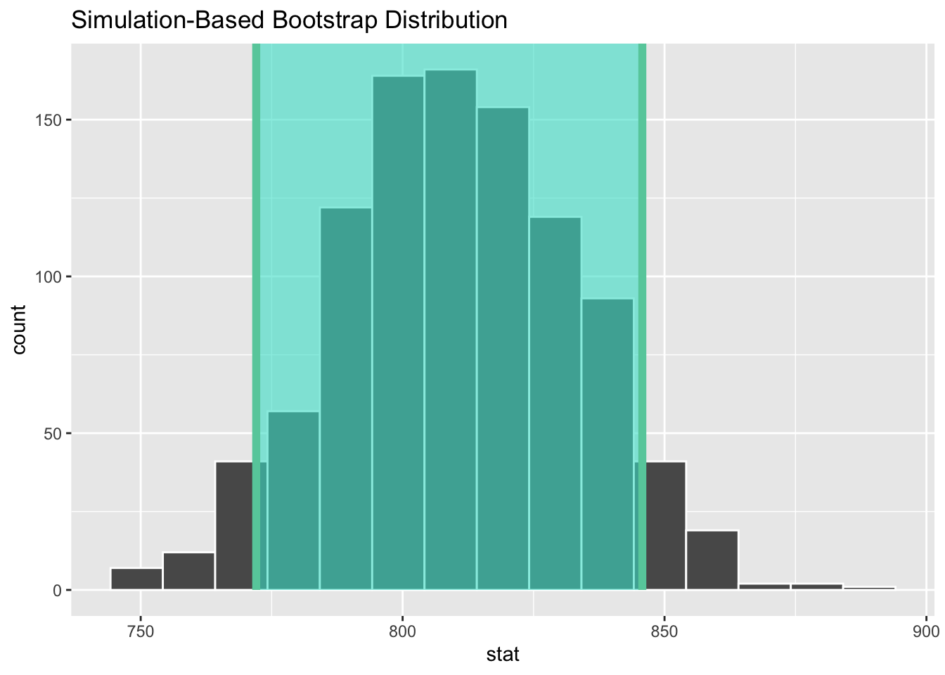

It is more narrow than the 95% confidence interval.

Difference in weight of Chipotle orders

We can calculate bootstrap confidence intervals for a range of statistical parameters.

Demo: Estimate a 95% confidence interval for the difference in means between orders placed by a person and those placed online.

# observed difference
d_hat <- chipotle |>
  specify(weight ~ order) |>
  calculate(stat = "diff in means", order = c("Person", "Online"))

# bootstrap CI
boot_diff_df <- chipotle |>
  specify(weight ~ order) |>
  generate(reps = 1000, type = "bootstrap") |>
  calculate(stat = "diff in means", order = c("Person", "Online"))

visualize(boot_diff_df) +
  shade_confidence_interval(endpoints = get_ci(x = boot_diff_df, level = 0.95))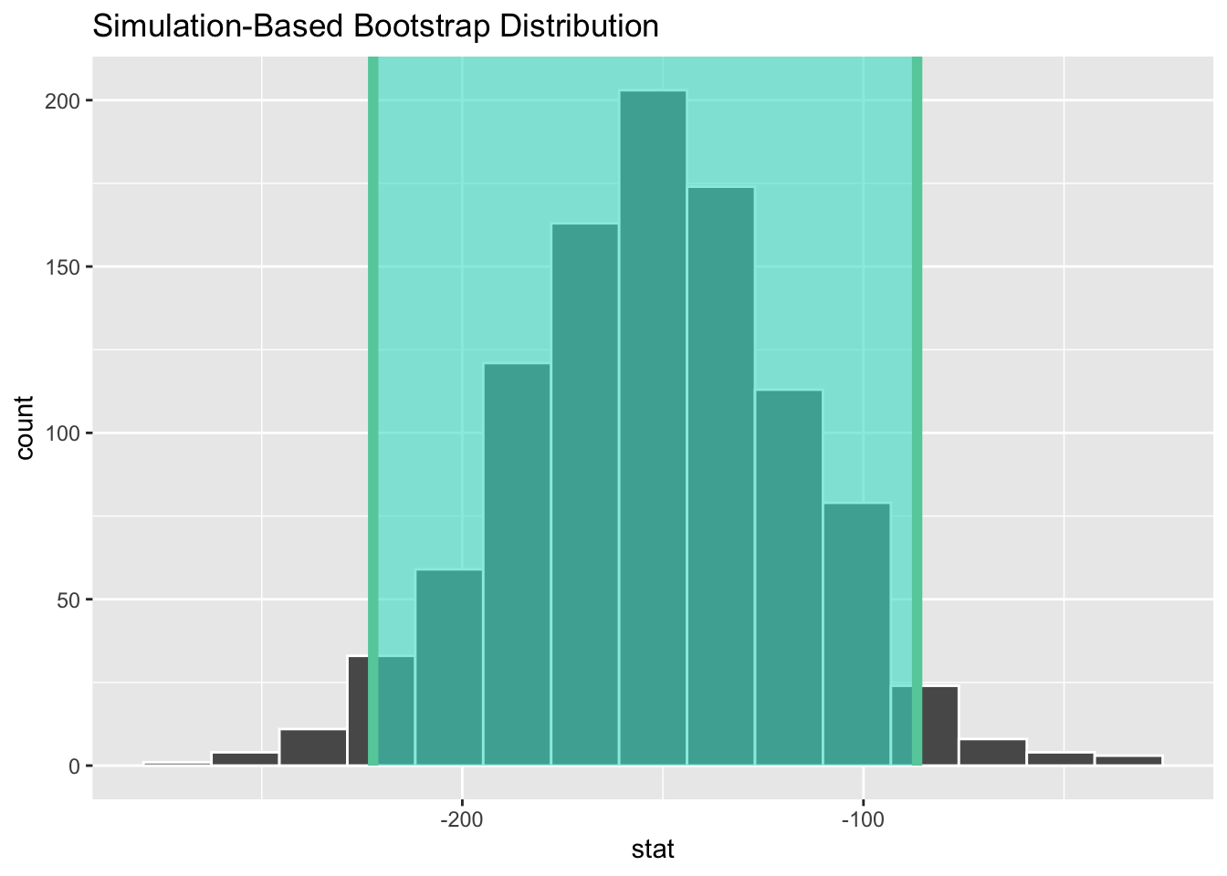

get_ci(x = boot_diff_df, level = 0.95)

# A tibble: 1 × 2
  lower_ci upper_ci
     <dbl>    <dbl>
1    -222.    -86.6

How does that compare to the \(p\)-value from our hypothesis test?

null_dist <- chipotle |>
  # specify the response and explanatory variable
  specify(weight ~ order) |>
  # declare the null hypothesis
  hypothesize(null = "independence") |>
  # simulate the null distribution
  generate(reps = 1000, type = "permute") |>
  # calculate the difference in means for each permutation
  calculate(stat = "diff in means", order = c("Person", "Online"))

# visualize simulated p-value
visualize(null_dist) +
  shade_p_value(obs_stat = d_hat, direction = "two-sided")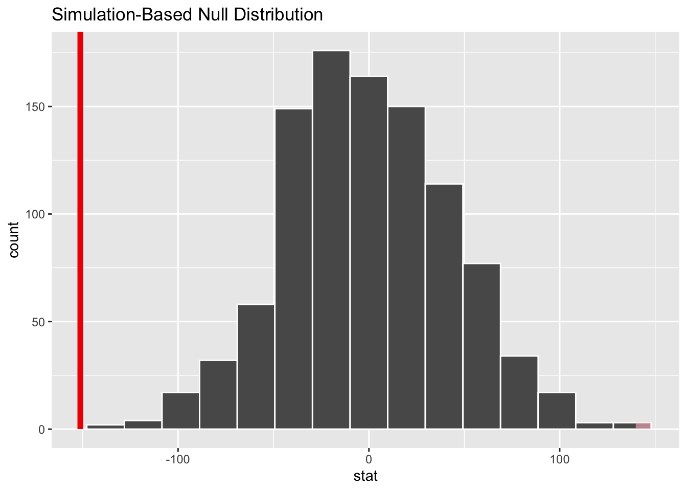

# calculate simulated p-value
null_dist |>
  get_p_value(obs_stat = d_hat, direction = "two-sided")

Warning: Please be cautious in reporting a p-value of 0. This result is an approximation
based on the number of `reps` chosen in the `generate()` step.
ℹ See `get_p_value()` (`?infer::get_p_value()`) for more information.

# A tibble: 1 × 1
  p_value
    <dbl>
1       0

Add response here. The \(p\)-value is less than \(0.05\), so the 95% confidence interval for the difference in means does not contain 0.

Multiple explanatory variables

We often calculate confidence intervals for the coefficients of multiple explanatory variables in a regression model. These can be useful in communicating our best guess as to the true value of the coefficient, and are often communicated as part of the results of a regression analysis.

Demo: Estimate the 95% confidence interval for the coefficients in the multiple variable model, and communicate them in a table and a coefficient plot.

# observed results
obs_fit <- chipotle |>
  specify(weight ~ order + meat + food + store) |>
  fit()

# null distribution for p-values
null_full_dist <- chipotle |>
  specify(weight ~ order + meat + food + store) |>
  hypothesize(null = "independence") |>
  generate(reps = 1000, type = "permute") |>
  fit()

p_vals <- get_p_value(null_full_dist, obs_stat = obs_fit, direction = "two-sided")

Warning: Please be cautious in reporting a p-value of 0. This result is an approximation
based on the number of `reps` chosen in the `generate()` step.
ℹ See `get_p_value()` (`?infer::get_p_value()`) for more information.

# bootstrap distribution for CIs
boot_full_dist <- chipotle |>
  specify(weight ~ order + meat + food + store) |>
  generate(reps = 1000, type = "bootstrap") |>
  fit()

# get 95% confidence interval
conf_ints <- get_ci(boot_full_dist, level = 0.95, point_estimate = obs_fit)

# visualize regression results using a results table
obs_fit |>
  # join with p-values
  left_join(p_vals) |>
  # join with confidence intervals
  left_join(conf_ints) |>
  # print an HTML table
  gt() |>
  # format for 2 significant digits
  fmt_number(
    columns = c(estimate, p_value, lower_ci, upper_ci),
    decimals = 2
  )

Joining with `by = join_by(term)`
Joining with `by = join_by(term)`

term	estimate	p_value	lower_ci	upper_ci
intercept	843.22	0.52	776.94	926.31
orderPerson	160.62	0.00	96.78	227.78
meatChicken	−29.47	0.50	−105.03	46.04
foodburrito	−82.38	0.06	−145.28	−15.81
storeStore 2	−62.26	0.23	−148.16	12.83
storeStore 3	−93.44	0.09	−173.17	−20.74

# visualize regression results using a coefficient plot
obs_fit |>
  # join with confidence intervals
  left_join(conf_ints) |>
  # order the coefficients by size, pull intercept to the beginning (by convention)
  mutate(term = fct_reorder(.f = term, .x = estimate) |>
           fct_relevel("intercept")) |>
  # draw a pointrange plot
  ggplot(mapping = aes(x = estimate, y = term, xmin = lower_ci, xmax = upper_ci)) +
  geom_pointrange() +
  # draw a vertical line at 0
  geom_vline(xintercept = 0, linetype = "dashed") +
  theme_minimal()

Joining with `by = join_by(term)`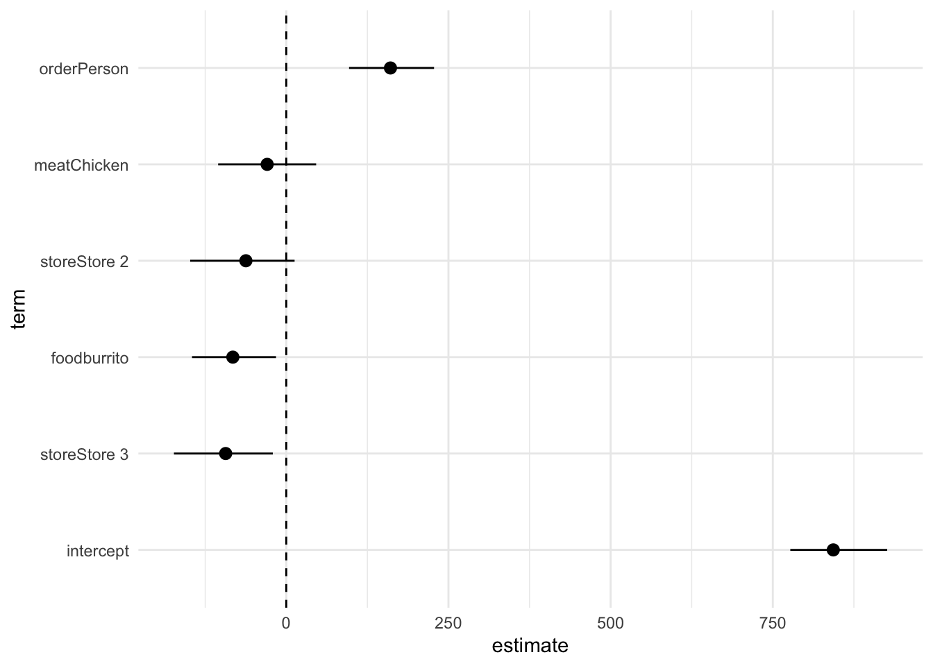

Session information

sessioninfo::session_info()

─ Session info ───────────────────────────────────────────────────────────────
 setting  value
 version  R version 4.4.2 (2024-10-31)
 os       macOS Sonoma 14.6.1
 system   aarch64, darwin20
 ui       X11
 language (EN)
 collate  en_US.UTF-8
 ctype    en_US.UTF-8
 tz       America/New_York
 date     2025-03-25
 pandoc   3.4 @ /usr/local/bin/ (via rmarkdown)

─ Packages ───────────────────────────────────────────────────────────────────
 package      * version    date (UTC) lib source
 archive        1.1.9      2024-09-12 [1] CRAN (R 4.4.1)
 backports      1.5.0      2024-05-23 [1] CRAN (R 4.4.0)
 base64enc      0.1-3      2015-07-28 [1] CRAN (R 4.3.0)
 bit            4.0.5      2022-11-15 [1] CRAN (R 4.3.0)
 bit64          4.0.5      2020-08-30 [1] CRAN (R 4.3.0)
 broom        * 1.0.6      2024-05-17 [1] CRAN (R 4.4.0)
 class          7.3-22     2023-05-03 [1] CRAN (R 4.4.2)
 cli            3.6.3      2024-06-21 [1] CRAN (R 4.4.0)
 codetools      0.2-20     2024-03-31 [1] CRAN (R 4.4.2)
 crayon         1.5.3      2024-06-20 [1] CRAN (R 4.4.0)
 data.table     1.15.4     2024-03-30 [1] CRAN (R 4.3.1)
 dials        * 1.3.0      2024-07-30 [1] CRAN (R 4.4.0)
 DiceDesign     1.10       2023-12-07 [1] CRAN (R 4.3.1)
 dichromat      2.0-0.1    2022-05-02 [1] CRAN (R 4.3.0)
 digest         0.6.37     2024-08-19 [1] CRAN (R 4.4.1)
 dplyr        * 1.1.4      2023-11-17 [1] CRAN (R 4.3.1)
 evaluate       1.0.3      2025-01-10 [1] CRAN (R 4.4.1)
 farver         2.1.2      2024-05-13 [1] CRAN (R 4.3.3)
 fastmap        1.2.0      2024-05-15 [1] CRAN (R 4.4.0)
 forcats      * 1.0.0      2023-01-29 [1] CRAN (R 4.3.0)
 foreach        1.5.2      2022-02-02 [1] CRAN (R 4.3.0)
 furrr          0.3.1      2022-08-15 [1] CRAN (R 4.3.0)
 future         1.33.2     2024-03-26 [1] CRAN (R 4.3.1)
 future.apply   1.11.2     2024-03-28 [1] CRAN (R 4.3.1)
 generics       0.1.3      2022-07-05 [1] CRAN (R 4.3.0)
 ggplot2      * 3.5.1      2024-04-23 [1] CRAN (R 4.3.1)
 globals        0.16.3     2024-03-08 [1] CRAN (R 4.3.1)
 glue           1.8.0      2024-09-30 [1] CRAN (R 4.4.1)
 gower          1.0.1      2022-12-22 [1] CRAN (R 4.3.0)
 GPfit          1.0-8      2019-02-08 [1] CRAN (R 4.3.0)
 gt           * 0.11.1     2024-10-04 [1] CRAN (R 4.4.1)
 gtable         0.3.6      2024-10-25 [1] CRAN (R 4.4.1)
 hardhat        1.4.0      2024-06-02 [1] CRAN (R 4.4.0)
 here           1.0.1      2020-12-13 [1] CRAN (R 4.3.0)
 hms            1.1.3      2023-03-21 [1] CRAN (R 4.3.0)
 htmltools      0.5.8.1    2024-04-04 [1] CRAN (R 4.3.1)
 htmlwidgets    1.6.4      2023-12-06 [1] CRAN (R 4.3.1)
 infer        * 1.0.7      2024-03-25 [1] CRAN (R 4.3.1)
 ipred          0.9-14     2023-03-09 [1] CRAN (R 4.3.0)
 iterators      1.0.14     2022-02-05 [1] CRAN (R 4.3.0)
 jsonlite       1.8.9      2024-09-20 [1] CRAN (R 4.4.1)
 knitr          1.49       2024-11-08 [1] CRAN (R 4.4.1)
 labeling       0.4.3      2023-08-29 [1] CRAN (R 4.3.0)
 lattice        0.22-6     2024-03-20 [1] CRAN (R 4.4.2)
 lava           1.8.0      2024-03-05 [1] CRAN (R 4.3.1)
 lhs            1.1.6      2022-12-17 [1] CRAN (R 4.3.0)
 lifecycle      1.0.4      2023-11-07 [1] CRAN (R 4.3.1)
 listenv        0.9.1      2024-01-29 [1] CRAN (R 4.3.1)
 lubridate    * 1.9.3      2023-09-27 [1] CRAN (R 4.3.1)
 magrittr       2.0.3      2022-03-30 [1] CRAN (R 4.3.0)
 MASS           7.3-61     2024-06-13 [1] CRAN (R 4.4.2)
 Matrix         1.7-1      2024-10-18 [1] CRAN (R 4.4.2)
 modeldata    * 1.4.0      2024-06-19 [1] CRAN (R 4.4.0)
 nnet           7.3-19     2023-05-03 [1] CRAN (R 4.4.2)
 parallelly     1.37.1     2024-02-29 [1] CRAN (R 4.3.1)
 parsnip      * 1.2.1      2024-03-22 [1] CRAN (R 4.3.1)
 pillar         1.10.1     2025-01-07 [1] CRAN (R 4.4.1)
 pkgconfig      2.0.3      2019-09-22 [1] CRAN (R 4.3.0)
 prodlim        2023.08.28 2023-08-28 [1] CRAN (R 4.3.0)
 purrr        * 1.0.2      2023-08-10 [1] CRAN (R 4.3.0)
 R6             2.5.1      2021-08-19 [1] CRAN (R 4.3.0)
 RColorBrewer   1.1-3      2022-04-03 [1] CRAN (R 4.3.0)
 Rcpp           1.0.14     2025-01-12 [1] CRAN (R 4.4.1)
 readr        * 2.1.5      2024-01-10 [1] CRAN (R 4.3.1)
 recipes      * 1.0.10     2024-02-18 [1] CRAN (R 4.3.1)
 repr           1.1.7      2024-03-22 [1] CRAN (R 4.4.0)
 rlang          1.1.5      2025-01-17 [1] CRAN (R 4.4.1)
 rmarkdown      2.29       2024-11-04 [1] CRAN (R 4.4.1)
 rpart          4.1.23     2023-12-05 [1] CRAN (R 4.4.2)
 rprojroot      2.0.4      2023-11-05 [1] CRAN (R 4.3.1)
 rsample      * 1.2.1      2024-03-25 [1] CRAN (R 4.3.1)
 rstudioapi     0.17.0     2024-10-16 [1] CRAN (R 4.4.1)
 sass           0.4.9      2024-03-15 [1] CRAN (R 4.3.1)
 scales       * 1.3.0.9000 2025-03-19 [1] Github (bensoltoff/scales@71d8f13)
 sessioninfo    1.2.2      2021-12-06 [1] CRAN (R 4.3.0)
 skimr        * 2.1.5      2022-12-23 [1] CRAN (R 4.3.0)
 stringi        1.8.4      2024-05-06 [1] CRAN (R 4.3.1)
 stringr      * 1.5.1      2023-11-14 [1] CRAN (R 4.3.1)
 survival       3.7-0      2024-06-05 [1] CRAN (R 4.4.2)
 tibble       * 3.2.1      2023-03-20 [1] CRAN (R 4.3.0)
 tidymodels   * 1.2.0      2024-03-25 [1] CRAN (R 4.3.1)
 tidyr        * 1.3.1      2024-01-24 [1] CRAN (R 4.3.1)
 tidyselect     1.2.1      2024-03-11 [1] CRAN (R 4.3.1)
 tidyverse    * 2.0.0      2023-02-22 [1] CRAN (R 4.3.0)
 timechange     0.3.0      2024-01-18 [1] CRAN (R 4.3.1)
 timeDate       4032.109   2023-12-14 [1] CRAN (R 4.3.1)
 tune         * 1.2.1      2024-04-18 [1] CRAN (R 4.3.1)
 tzdb           0.4.0      2023-05-12 [1] CRAN (R 4.3.0)
 vctrs          0.6.5      2023-12-01 [1] CRAN (R 4.3.1)
 vroom          1.6.5      2023-12-05 [1] CRAN (R 4.3.1)
 withr          3.0.2      2024-10-28 [1] CRAN (R 4.4.1)
 workflows    * 1.1.4      2024-02-19 [1] CRAN (R 4.4.0)
 workflowsets * 1.1.0      2024-03-21 [1] CRAN (R 4.3.1)
 xfun           0.50.5     2025-01-15 [1] https://yihui.r-universe.dev (R 4.4.2)
 xml2           1.3.6      2023-12-04 [1] CRAN (R 4.3.1)
 yaml           2.3.10     2024-07-26 [1] CRAN (R 4.4.0)
 yardstick    * 1.3.1      2024-03-21 [1] CRAN (R 4.3.1)

 [1] /Library/Frameworks/R.framework/Versions/4.4-arm64/Resources/library

──────────────────────────────────────────────────────────────────────────────