AE 14: Do you get more food when you order in-person at Chipotle?
Inspired by this Reddit post, we will conduct a hypothesis test to determine if there is a difference in the weight of Chipotle orders between in-person and online orders. The data was originally collected by Zackary Smigel, and a cleaned copy be found in data/chipotle.csv.
Throughout the application exercise we will use the {infer} package which is part of {tidymodels} to conduct our permutation tests.
skim(chipotle)| Name | chipotle |
| Number of rows | 30 |
| Number of columns | 7 |
| _______________________ | |
| Column type frequency: | |
| character | 4 |
| Date | 1 |
| numeric | 2 |
| ________________________ | |
| Group variables | None |
Variable type: character
| skim_variable | n_missing | complete_rate | min | max | empty | n_unique | whitespace |
|---|---|---|---|---|---|---|---|
| order | 0 | 1 | 6 | 6 | 0 | 2 | 0 |
| meat | 0 | 1 | 7 | 8 | 0 | 2 | 0 |
| store | 0 | 1 | 7 | 7 | 0 | 3 | 0 |
| food | 0 | 1 | 4 | 7 | 0 | 2 | 0 |
Variable type: Date
| skim_variable | n_missing | complete_rate | min | max | median | n_unique |
|---|---|---|---|---|---|---|
| date | 0 | 1 | 2024-01-12 | 2024-02-10 | 2024-01-26 | 30 |
Variable type: numeric
| skim_variable | n_missing | complete_rate | mean | sd | p0 | p25 | p50 | p75 | p100 | hist |
|---|---|---|---|---|---|---|---|---|---|---|
| day | 0 | 1 | 15.5 | 8.80 | 1.00 | 8.25 | 15.50 | 22.75 | 30.00 | ▇▇▇▇▇ |
| weight | 0 | 1 | 810.8 | 123.37 | 510.29 | 715.82 | 793.79 | 907.18 | 1048.93 | ▁▆▇▇▂ |
The variable we will use in this analysis is weight which records the total weight of the meal in grams.
Hypotheses
We wish to test the claim that the difference in weight between in-person and online orders must be due to something other than chance.
ggplot(data = chipotle, aes(x = weight, color = order)) +
  geom_density() +
  labs(
    title = "Chipotle Weight Distribution",
    x = "Weight (g)",
    y = "Count"
  )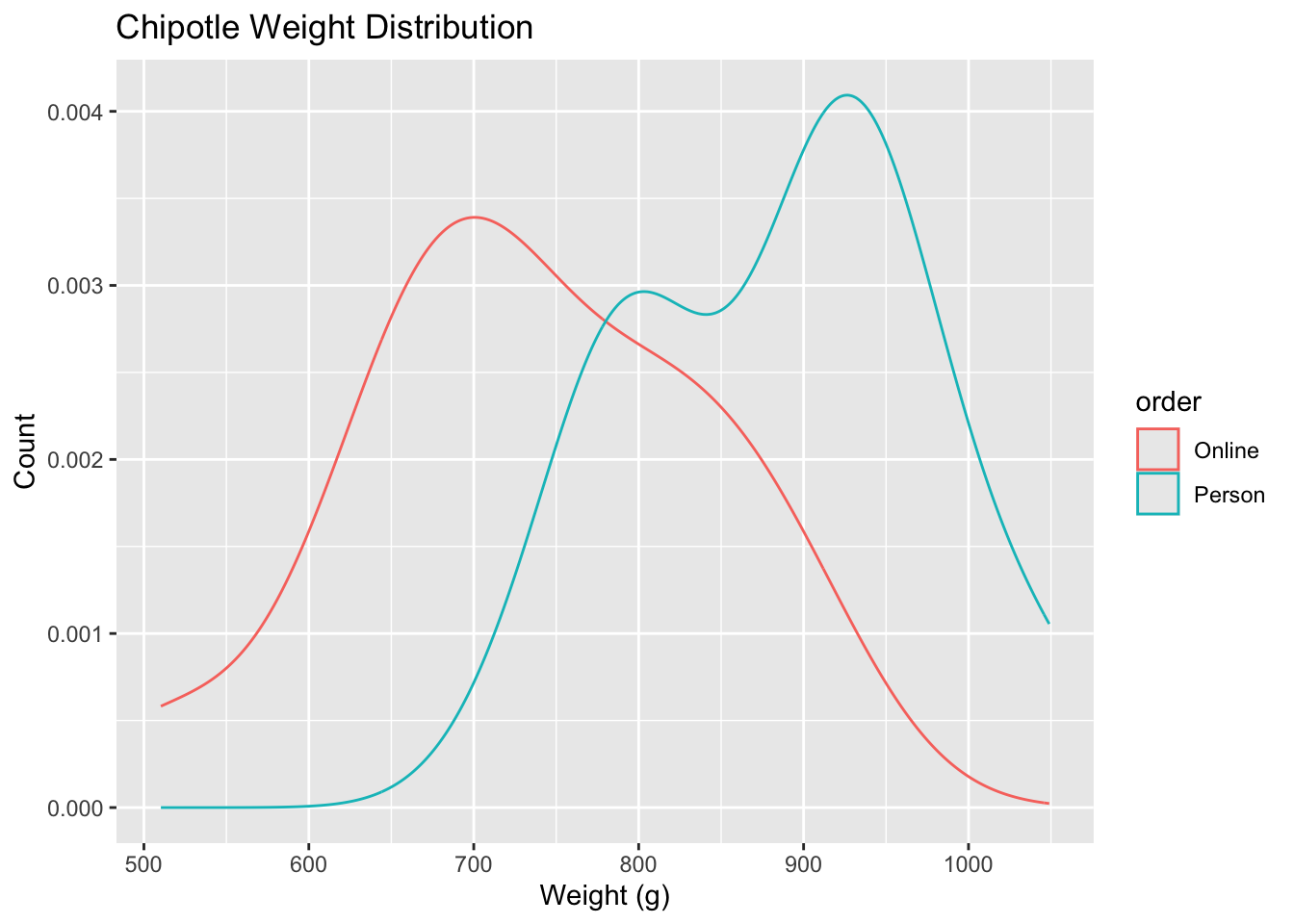
- Your turn: Write out the correct null and alternative hypothesis in terms of the difference in means between in-person and online orders. Do this in both words and in proper notation.
Null hypothesis: TODO
\[H_0: \mu_{\text{in-person}} - \mu_{\text{online}} = TODO\]
Alternative hypothesis: TODO
\[H_A: \mu_{\text{in-person}} - \mu_{\text{online}} TODO\]
Observed data
Our goal is to use the collected data and calculate the probability of a sample statistic at least as extreme as the one observed in our data if in fact the null hypothesis is true.
- Demo: Calculate and report the sample statistic below using proper notation.
The null distribution
Let’s use permutation-based methods to conduct the hypothesis test specified above.
Generate
We’ll start by generating the null distribution.
- Demo: Generate the null distribution.
set.seed(123)null_dist <- chipotle |>
# specify the response and explanatory variable
specify(weight ~ order) |>
# declare the null hypothesis
hypothesize(null = "independence") |>
# simulate the null distribution
generate(reps = 1000, type = "permute") |>
# calculate the difference in means for each permutation
calculate(stat = "diff in means", order = c("Person", "Online"))-
Your turn: Take a look at
null_dist. What does each element in this distribution represent?
null_distResponse: weight (numeric)
Explanatory: order (factor)
Null Hypothesis: indep...
# A tibble: 1,000 × 2
replicate stat
<int> <dbl>
1 1 -68.0
2 2 37.8
3 3 15.1
4 4 -30.2
5 5 37.8
6 6 -3.78
7 7 -56.7
8 8 26.5
9 9 -37.8
10 10 45.4
# ℹ 990 more rowsAdd response here.
Visualize
-
Question: Before you visualize the distribution of
null_dist– at what value would you expect this distribution to be centered? Why?Add response here.
Demo: Create an appropriate visualization for your null distribution. Does the center of the distribution match what you guessed in the previous question?
visualize(null_dist)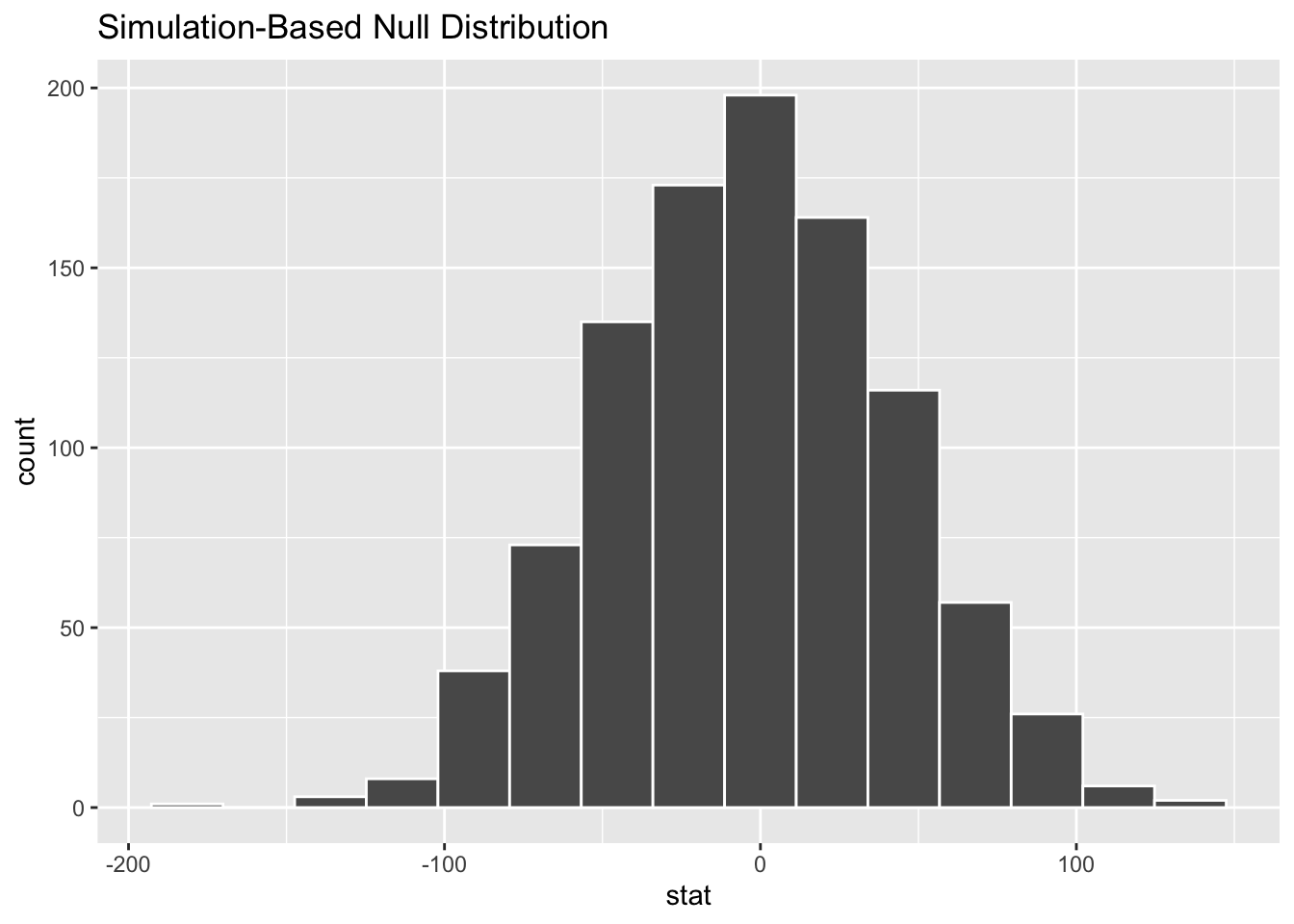
- Demo: Now, add a vertical red line on your null distribution that represents your sample statistic.
visualize(null_dist) +
  geom_vline(xintercept = 151, color = "red")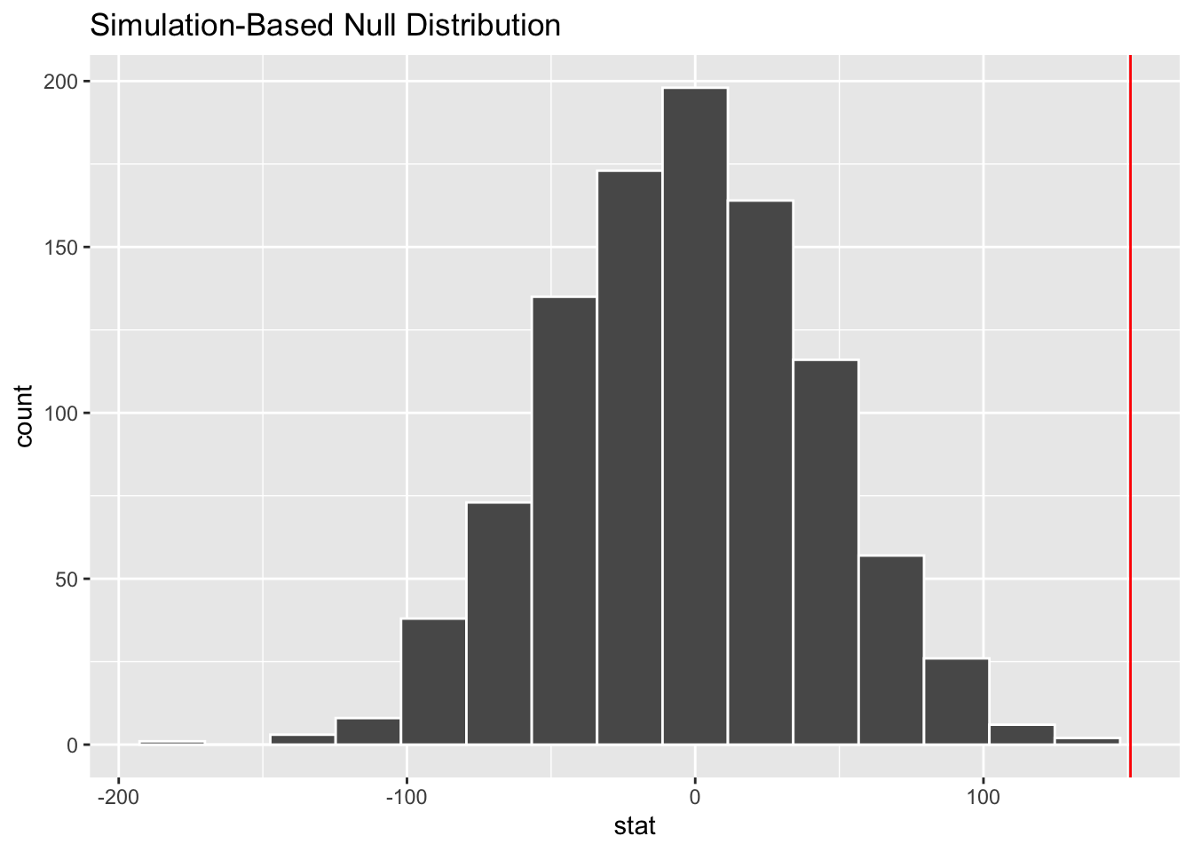
-
Question: Based on the position of this line, does your observed sample difference in means appear to be an unusual observation under the assumption of the null hypothesis?
Add response here.
p-value
Above, we eyeballed how likely/unlikely our observed mean is. Now, let’s actually quantify it using a p-value.
-
Question: What is a p-value?
Add response here.
Guesstimate the p-value
- Demo: Visualize the p-value.
visualize(null_dist) +
  geom_vline(xintercept = 151, color = "red") +
  geom_vline(xintercept = -151, color = "red", linetype = "dashed")
-
Your turn: What is you guesstimate of the p-value?
Add response here.
Calculate the p-value
# calculate sample statistic
d_hat <- chipotle |>
  specify(weight ~ order) |>
  # calculate the observed difference in means
  calculate(stat = "diff in means", order = c("Person", "Online"))

# visualize simulated p-value
visualize(null_dist) +
  shade_p_value(obs_stat = d_hat, direction = "two-sided")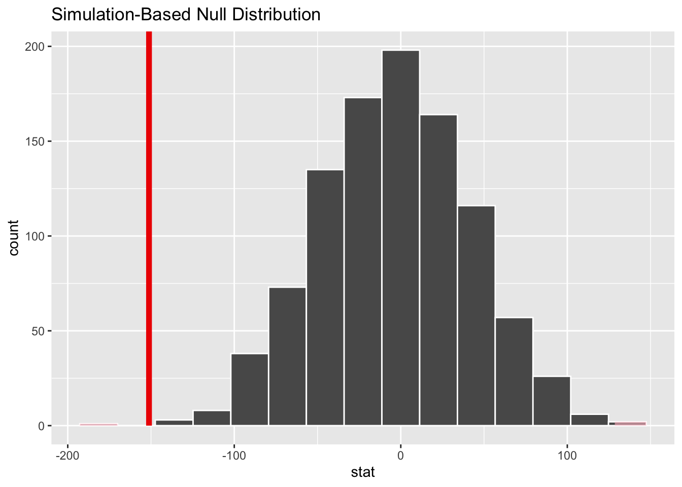
# calculate simulated p-value
null_dist |>
  get_p_value(obs_stat = d_hat, direction = "two-sided")
# A tibble: 1 × 1
p_value
<dbl>
1 0.002Conclusion
-
Your turn: What is the conclusion of the hypothesis test based on the p-value you calculated? Make sure to frame it in context of the data and the research question. Use a significance level of 5% to make your conclusion.
Add response here.
-
Demo: Interpret the p-value in context of the data and the research question.
Add response here.
Reframe as a linear regression model
While we originally evaluated the null/alternative hypotheses as a difference in means, we could also frame this as a regression problem where the outcome of interest (weight of the order) is a continuous variable.1 Framing it this way allows us to include additional explanatory variables in our model which may account for some of the variation in weight.
Single explanatory variable
Demo: Let’s reevaluate the original hypotheses using a linear regression model. Notice the similarities and differences in the code compared to a difference in means, and that the obtained p-value should be nearly identical to the results from the difference in means test.
# observed fit
obs_fit <- chipotle |>
  # specify the response and explanatory variable
  specify(weight ~ order) |>
  # fit the linear regression model
  fit()

# null distribution
set.seed(123)

null_dist <- chipotle |>
  # specify the response and explanatory variable
  specify(weight ~ order) |>
  # declare the null hypothesis
  hypothesize(null = "independence") |>
  # simulate the null distribution
  generate(reps = 1000, type = "permute") |>
  # estimate the linear regression model for each permutation
  fit()

# examine p-value
visualize(null_dist) +
  shade_p_value(obs_stat = obs_fit, direction = "two-sided")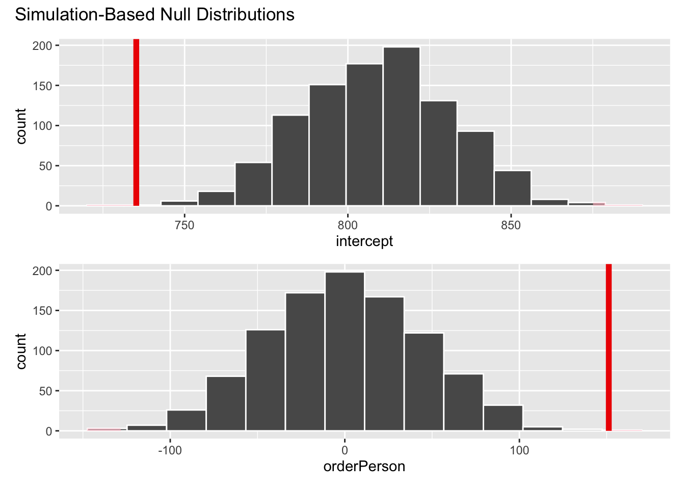
# calculate p-value
null_dist |>
  get_p_value(obs_stat = obs_fit, direction = "two-sided")
# A tibble: 2 × 2
term p_value
<chr> <dbl>
1 intercept 0.002
2 orderPerson 0.002Multiple explanatory variables
Demo: Now let’s also account for additional variables that likely influence the weight of the order.
- Protein type (
meat) - Type of meal (
food) - burrito or bowl - Store (
store) - at which Chipotle location the order was placed
# observed results
obs_fit <- chipotle |>
  specify(weight ~ order + meat + food + store) |>
  fit()

# permutation null distribution
null_dist <- chipotle |>
  specify(weight ~ order + meat + food + store) |>
  hypothesize(null = "independence") |>
  generate(reps = 1000, type = "permute") |>
  fit()

# examine p-value
visualize(null_dist) +
  shade_p_value(obs_stat = obs_fit, direction = "two-sided")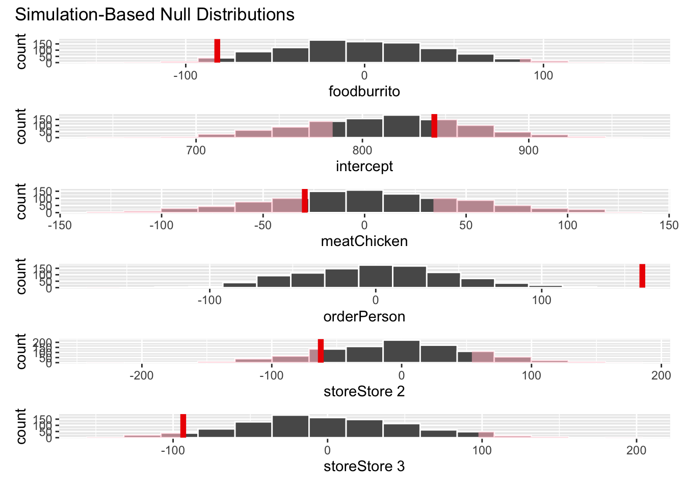
null_dist |>
  get_p_value(obs_stat = obs_fit, direction = "two-sided")
Warning: Please be cautious in reporting a p-value of 0. This result is an approximation
based on the number of `reps` chosen in the `generate()` step.
ℹ See `get_p_value()` (`?infer::get_p_value()`) for more information.# A tibble: 6 × 2
term p_value
<chr> <dbl>
1 foodburrito 0.054
2 intercept 0.54
3 meatChicken 0.51
4 orderPerson 0
5 storeStore 2 0.31
6 storeStore 3 0.078-
Your turn: What is the conclusion of the hypothesis test based on the p-value you calculated? Make sure to frame it in context of the data and the research question. Use a significance level of 5% to make your conclusion.
Add response here.
-
Your turn: Interpret the p-value for the order in context of the data and the research question.
Add response here.
Footnotes
We will cover linear regression in more detail next week. It can be shown that under certain conditions linear regression is equivalent to a difference of means test.↩︎