AE 04: Joining prognosticators
Suggested answers
Application exercise
Answers
Important
These are suggested answers. This document should be used as reference only, it’s not designed to be an exhaustive key.
Prognosticator success
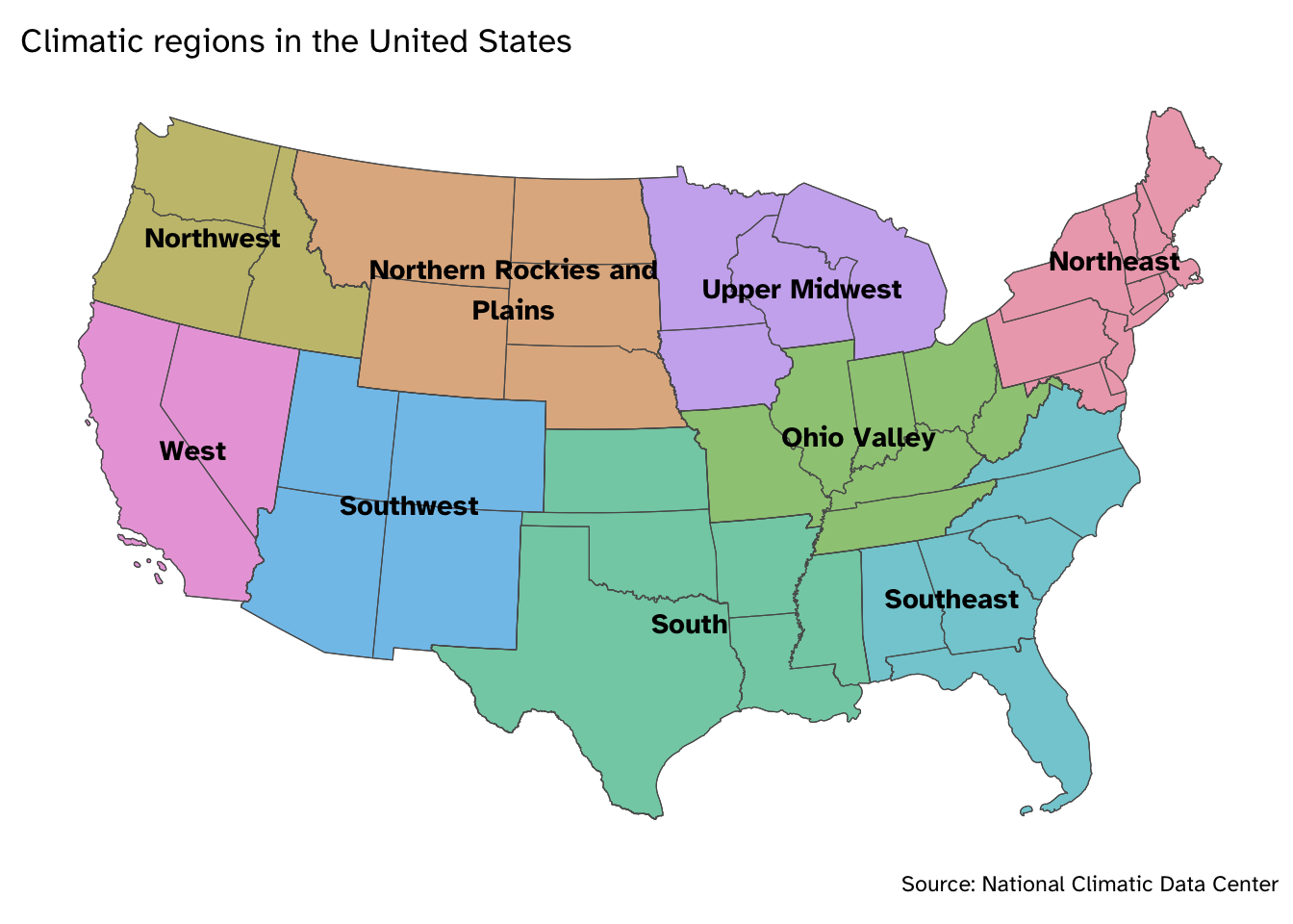
We previously examined the accuracy rate of Groundhog Day prognosticators.1 Today we want to work with the original dataset to understand how those accuracy metrics were generated and answer the question: How does prognosticator accuracy vary by climatic region?
1 See ae-02
Let’s start by looking at the seers data frame.
glimpse(seers)Rows: 1,710
Columns: 7
$ name <chr> "Punxsutawney Phil", "Punxsutawney Phil", "Punxsutawne…
$ forecaster_type <chr> "Groundhog", "Groundhog", "Groundhog", "Groundhog", "G…
$ alive <lgl> TRUE, TRUE, TRUE, TRUE, TRUE, TRUE, TRUE, TRUE, TRUE, …
$ town <chr> "Punxsutawney", "Punxsutawney", "Punxsutawney", "Punxs…
$ state <chr> "PA", "PA", "PA", "PA", "PA", "PA", "PA", "PA", "PA", …
$ year <dbl> 2024, 2023, 2022, 2021, 2020, 2019, 2018, 2017, 2016, …
$ prediction <chr> "Early Spring", "Late Winter", "Late Winter", "Late Wi…We have the predictions, but our goal is to make a visualization by climate region.2
Join the data frames
Let’s take a look at the weather data frame.
glimpse(weather)Rows: 5,568
Columns: 13
$ region <chr> "Northeast", "Northeast", "Northeast", "Northeast", "No…
$ state_abb <chr> "CT", "CT", "CT", "CT", "CT", "CT", "CT", "CT", "CT", "…
$ id <dbl> 101, 101, 101, 101, 101, 101, 101, 101, 101, 101, 101, …
$ year <dbl> 1909, 1910, 1911, 1912, 1913, 1914, 1915, 1916, 1917, 1…
$ avg_temp <dbl> 28.00, 29.20, 24.90, 23.15, 28.05, 22.05, 27.50, 21.55,…
$ temp_hist <dbl> 25.58333, 26.09000, 26.16667, 25.85667, 25.63333, 25.52…
$ temp_hist_sd <dbl> 4.245360, 4.241218, 4.103158, 4.124311, 3.907804, 4.016…
$ temp_sd <dbl> 4.154767, 4.154767, 4.154767, 4.154767, 4.154767, 4.154…
$ precip <dbl> 4.005, 2.520, 2.810, 3.570, 3.765, 2.920, 2.330, 3.425,…
$ precip_hist <dbl> 3.476667, 3.526667, 3.378000, 3.411000, 3.446333, 3.352…
$ precip_hist_sd <dbl> 1.1784719, 1.2081292, 1.1442431, 1.1620681, 1.2039309, …
$ precip_sd <dbl> 0.9715631, 0.9715631, 0.9715631, 0.9715631, 0.9715631, …
$ outcome <chr> "Early Spring", "Early Spring", "Early Spring", "Late W…-
Your turn (2 minutes):
- Which variable(s) will we use to join the
seersandweatherdata frames? - We want to keep all rows and columns from
seersand add columns for corresponding weather data. Which join function should we use?
- Which variable(s) will we use to join the
-
Demo: Join the two data frames and assign the joined data frame to
seers_weather.
seers_weather <- inner_join(
  x = seers, y = weather,
  by = join_by(state == state_abb, year)
)
Calculate the variables
-
Demo: Take a look at the updated
seersdata frame. First we need to calculate for each prediction whether or not the prognostication was correct.
seers_weather <- seers_weather |>
mutate(correct_pred = prediction == outcome)-
Demo: Calculate the accuracy rate (we’ll call it
preds_rate) for weather predictions using thesummarize()function in {dplyr}. Note that the function for calculating the mean ismean()in R.
seers_weather |> # start with seers data frame
  group_by(region) |> # group by region
  summarize(preds_rate = mean(correct_pred)) # calculate accuracy rate
# A tibble: 9 × 2
region preds_rate
<chr> <dbl>
1 Northeast 0.491
2 Northern Rockies and Plains 0.574
3 Northwest 0.442
4 Ohio Valley 0.557
5 South 0.506
6 Southeast 0.568
7 Southwest 0.667
8 Upper Midwest 0.5
9 West 0.286-
Your turn (5 minutes): Now expand your calculations to also calculate the number of predictions in each region and the standard error of accuracy rate. Store this data frame as
seers_summary. Recall the formula for the standard error of a sample proportion:
\[SE(\hat{p}) \approx \sqrt{\frac{(\hat{p})(1 - \hat{p})}{n}}\]
seers_summary <- seers_weather |>
  group_by(region) |>
  summarize(
    preds_rate = mean(correct_pred),
    preds_n = n(),
    preds_se = sqrt((preds_rate * (1 - preds_rate)) / preds_n)
  )
seers_summary
# A tibble: 9 × 4
region preds_rate preds_n preds_se
<chr> <dbl> <int> <dbl>
1 Northeast 0.491 696 0.0189
2 Northern Rockies and Plains 0.574 47 0.0721
3 Northwest 0.442 52 0.0689
4 Ohio Valley 0.557 280 0.0297
5 South 0.506 79 0.0562
6 Southeast 0.568 176 0.0373
7 Southwest 0.667 36 0.0786
8 Upper Midwest 0.5 104 0.0490
9 West 0.286 7 0.171 -
Demo: Take the
seers_summarydata frame and order the results in descending order of accuracy rate.
seers_summary |> # start with seers_summary data frame
  arrange(desc(preds_rate)) # order in descending order of preds_rate
# A tibble: 9 × 4
region preds_rate preds_n preds_se
<chr> <dbl> <int> <dbl>
1 Southwest 0.667 36 0.0786
2 Northern Rockies and Plains 0.574 47 0.0721
3 Southeast 0.568 176 0.0373
4 Ohio Valley 0.557 280 0.0297
5 South 0.506 79 0.0562
6 Upper Midwest 0.5 104 0.0490
7 Northeast 0.491 696 0.0189
8 Northwest 0.442 52 0.0689
9 West 0.286 7 0.171 Recreate the plot
- Demo: Recreate the following plot using the data frame you have developed so far.
seers_summary |>
  mutate(region = fct_reorder(.f = region, .x = preds_rate)) |>
  ggplot(mapping = aes(x = preds_rate, y = region)) +
  geom_point(mapping = aes(size = preds_n)) +
  geom_linerange(mapping = aes(
    xmin = preds_rate - preds_se,
    xmax = preds_rate + preds_se
  )) +
  scale_x_continuous(labels = label_percent()) +
  labs(
    title = "Prognosticator accuracy rate for late winter/early spring",
    subtitle = "By climate region",
    x = "Prediction accuracy",
    y = NULL,
    size = "Total number\nof predictions",
    caption = "Source: Countdown to Groundhog Day & NOAA"
  ) +
  theme_minimal()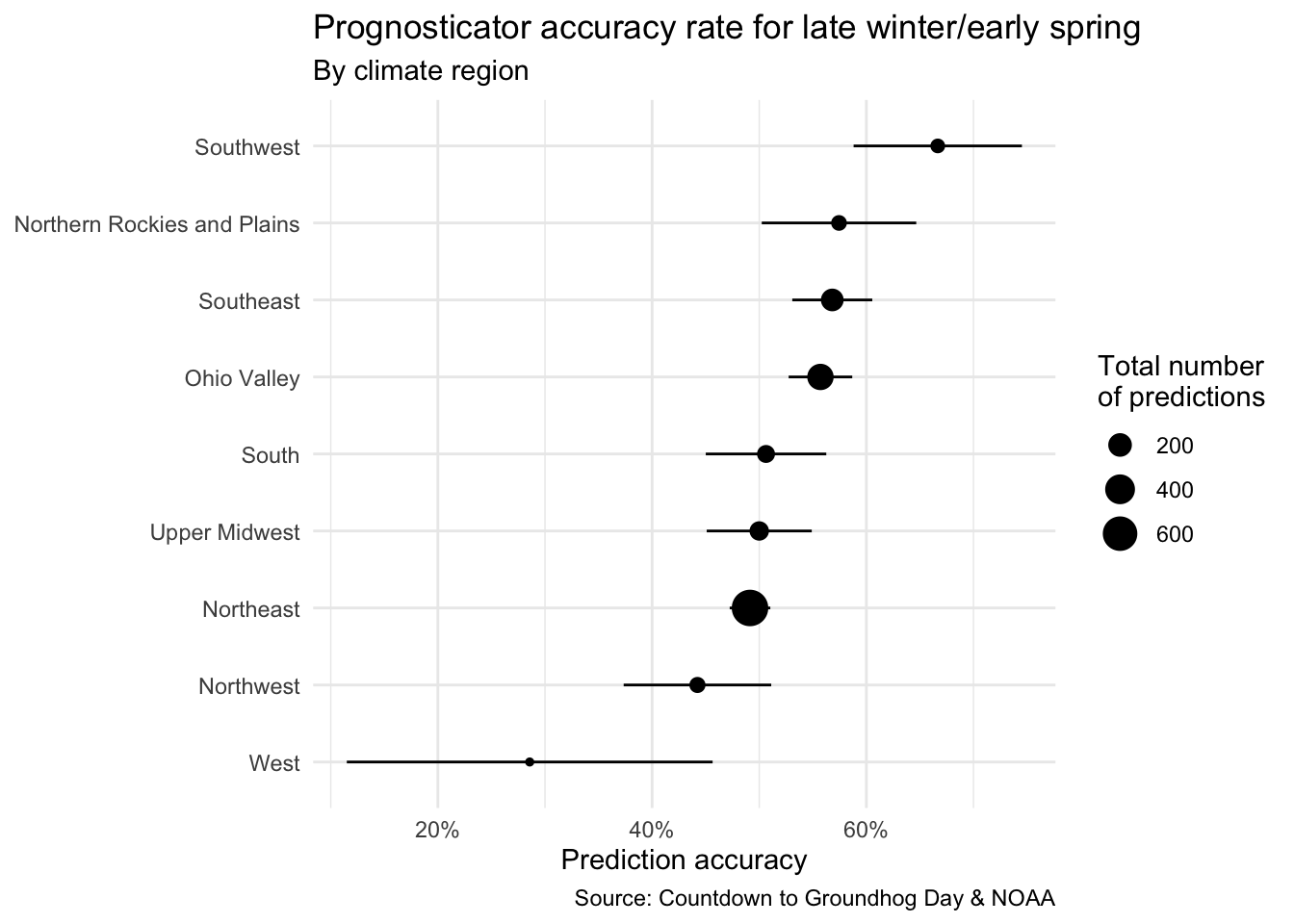
- Your turn (time permitting): Make any other changes you would like to improve it.
# add your code here
Session information
sessioninfo::session_info()─ Session info ───────────────────────────────────────────────────────────────
setting value
version R version 4.4.2 (2024-10-31)
os macOS Sonoma 14.6.1
system aarch64, darwin20
ui X11
language (EN)
collate en_US.UTF-8
ctype en_US.UTF-8
tz America/New_York
date 2025-02-13
pandoc 3.4 @ /usr/local/bin/ (via rmarkdown)
─ Packages ───────────────────────────────────────────────────────────────────
package * version date (UTC) lib source
archive 1.1.9 2024-09-12 [1] CRAN (R 4.4.1)
bit 4.0.5 2022-11-15 [1] CRAN (R 4.3.0)
bit64 4.0.5 2020-08-30 [1] CRAN (R 4.3.0)
cli 3.6.3 2024-06-21 [1] CRAN (R 4.4.0)
crayon 1.5.3 2024-06-20 [1] CRAN (R 4.4.0)
dichromat 2.0-0.1 2022-05-02 [1] CRAN (R 4.3.0)
digest 0.6.37 2024-08-19 [1] CRAN (R 4.4.1)
dplyr * 1.1.4 2023-11-17 [1] CRAN (R 4.3.1)
evaluate 1.0.3 2025-01-10 [1] CRAN (R 4.4.1)
farver 2.1.2 2024-05-13 [1] CRAN (R 4.3.3)
fastmap 1.2.0 2024-05-15 [1] CRAN (R 4.4.0)
forcats * 1.0.0 2023-01-29 [1] CRAN (R 4.3.0)
generics 0.1.3 2022-07-05 [1] CRAN (R 4.3.0)
ggplot2 * 3.5.1 2024-04-23 [1] CRAN (R 4.3.1)
glue 1.8.0 2024-09-30 [1] CRAN (R 4.4.1)
gtable 0.3.6 2024-10-25 [1] CRAN (R 4.4.1)
here 1.0.1 2020-12-13 [1] CRAN (R 4.3.0)
hms 1.1.3 2023-03-21 [1] CRAN (R 4.3.0)
htmltools 0.5.8.1 2024-04-04 [1] CRAN (R 4.3.1)
htmlwidgets 1.6.4 2023-12-06 [1] CRAN (R 4.3.1)
jsonlite 1.8.9 2024-09-20 [1] CRAN (R 4.4.1)
knitr 1.49 2024-11-08 [1] CRAN (R 4.4.1)
labeling 0.4.3 2023-08-29 [1] CRAN (R 4.3.0)
lifecycle 1.0.4 2023-11-07 [1] CRAN (R 4.3.1)
lubridate * 1.9.3 2023-09-27 [1] CRAN (R 4.3.1)
magrittr 2.0.3 2022-03-30 [1] CRAN (R 4.3.0)
pillar 1.10.1 2025-01-07 [1] CRAN (R 4.4.1)
pkgconfig 2.0.3 2019-09-22 [1] CRAN (R 4.3.0)
purrr * 1.0.2 2023-08-10 [1] CRAN (R 4.3.0)
R6 2.5.1 2021-08-19 [1] CRAN (R 4.3.0)
ragg 1.3.2 2024-05-15 [1] CRAN (R 4.4.0)
RColorBrewer 1.1-3 2022-04-03 [1] CRAN (R 4.3.0)
readr * 2.1.5 2024-01-10 [1] CRAN (R 4.3.1)
rlang 1.1.5 2025-01-17 [1] CRAN (R 4.4.1)
rmarkdown 2.29 2024-11-04 [1] CRAN (R 4.4.1)
rprojroot 2.0.4 2023-11-05 [1] CRAN (R 4.3.1)
rstudioapi 0.17.0 2024-10-16 [1] CRAN (R 4.4.1)
scales * 1.3.0.9000 2024-11-14 [1] Github (r-lib/scales@ee03582)
sessioninfo 1.2.2 2021-12-06 [1] CRAN (R 4.3.0)
stringi 1.8.4 2024-05-06 [1] CRAN (R 4.3.1)
stringr * 1.5.1 2023-11-14 [1] CRAN (R 4.3.1)
systemfonts 1.2.0 2025-01-16 [1] CRAN (R 4.4.1)
textshaping 0.4.0 2024-05-24 [1] CRAN (R 4.4.0)
tibble * 3.2.1 2023-03-20 [1] CRAN (R 4.3.0)
tidyr * 1.3.1 2024-01-24 [1] CRAN (R 4.3.1)
tidyselect 1.2.1 2024-03-11 [1] CRAN (R 4.3.1)
tidyverse * 2.0.0 2023-02-22 [1] CRAN (R 4.3.0)
timechange 0.3.0 2024-01-18 [1] CRAN (R 4.3.1)
tzdb 0.4.0 2023-05-12 [1] CRAN (R 4.3.0)
utf8 1.2.4 2023-10-22 [1] CRAN (R 4.3.1)
vctrs 0.6.5 2023-12-01 [1] CRAN (R 4.3.1)
vroom 1.6.5 2023-12-05 [1] CRAN (R 4.3.1)
withr 3.0.2 2024-10-28 [1] CRAN (R 4.4.1)
xfun 0.50.5 2025-01-15 [1] https://yihui.r-universe.dev (R 4.4.2)
yaml 2.3.10 2024-07-26 [1] CRAN (R 4.4.0)
[1] /Library/Frameworks/R.framework/Versions/4.4-arm64/Resources/library
──────────────────────────────────────────────────────────────────────────────