Formatting results tables
There are many great resources for creating summary results tables in R. If you search online you’ll find dozens of packages and tutorials showing you how to create beautiful tables. This tutorial shows just a small fraction of options.
Summary statistics
Don’t do this
skim(chipotle)| Name | chipotle |
| Number of rows | 30 |
| Number of columns | 7 |
| _______________________ | |
| Column type frequency: | |
| character | 4 |
| Date | 1 |
| numeric | 2 |
| ________________________ | |
| Group variables | None |
Variable type: character
| skim_variable | n_missing | complete_rate | min | max | empty | n_unique | whitespace |
|---|---|---|---|---|---|---|---|
| order | 0 | 1 | 6 | 6 | 0 | 2 | 0 |
| meat | 0 | 1 | 7 | 8 | 0 | 2 | 0 |
| store | 0 | 1 | 7 | 7 | 0 | 3 | 0 |
| food | 0 | 1 | 4 | 7 | 0 | 2 | 0 |
Variable type: Date
| skim_variable | n_missing | complete_rate | min | max | median | n_unique |
|---|---|---|---|---|---|---|
| date | 0 | 1 | 2024-01-12 | 2024-02-10 | 2024-01-26 | 30 |
Variable type: numeric
| skim_variable | n_missing | complete_rate | mean | sd | p0 | p25 | p50 | p75 | p100 | hist |
|---|---|---|---|---|---|---|---|---|---|---|
| day | 0 | 1 | 15.5 | 8.80 | 1.00 | 8.25 | 15.50 | 22.75 | 30.00 | ▇▇▇▇▇ |
| weight | 0 | 1 | 810.8 | 123.37 | 510.29 | 715.82 | 793.79 | 907.18 | 1048.93 | ▁▆▇▇▂ |
skim() is great for exploratory analysis - not for presenting results in a published document.
Do this instead
{gtsummary} has functions for calculating descriptive statistics and formatting them nicely in a table.
chipotle |>
  # select columns to summarize
  select(order:weight) |>
  # use gtsummary::tbl_summary()
tbl_summary()| Characteristic | N = 301 |
|---|---|
| order | |
| Online | 15 (50%) |
| Person | 15 (50%) |
| meat | |
| Carnitas | 10 (33%) |
| Chicken | 20 (67%) |
| store | |
| Store 1 | 10 (33%) |
| Store 2 | 10 (33%) |
| Store 3 | 10 (33%) |
| food | |
| bowl | 15 (50%) |
| burrito | 15 (50%) |
| weight | 794 (709, 907) |
| 1 n (%); Median (Q1, Q3) | |
# by group
chipotle |>
  select(order:weight) |>
  tbl_summary(
    by = order,
    # include human readable labels for variables
    label = list(
      meat = "Meat",
      store = "Store",
      food = "Meal type",
      weight = "Weight (grams)"
    )
)| Characteristic |
Online N = 151 |
Person N = 151 |
|---|---|---|
| Meat | ||
| Carnitas | 6 (40%) | 4 (27%) |
| Chicken | 9 (60%) | 11 (73%) |
| Store | ||
| Store 1 | 5 (33%) | 5 (33%) |
| Store 2 | 5 (33%) | 5 (33%) |
| Store 3 | 5 (33%) | 5 (33%) |
| Meal type | ||
| bowl | 8 (53%) | 7 (47%) |
| burrito | 7 (47%) | 8 (53%) |
| Weight (grams) | 709 (652, 822) | 907 (794, 936) |
| 1 n (%); Median (Q1, Q3) | ||
The tbl_summary() tutorial includes many examples of how to generate and customize summary tables.
Linear regression model
Don’t do this
Say you estimate a linear regression model to predict the weight of each order based on the order type, meat type, food type, and store. You might report the results like this:
# observed results
obs_fit <- chipotle |>
  specify(weight ~ order + meat + food + store) |>
  fit()

# null distribution for p-values
null_full_dist <- chipotle |>
  specify(weight ~ order + meat + food + store) |>
  hypothesize(null = "independence") |>
  generate(reps = 1000, type = "permute") |>
  fit()

p_vals <- get_p_value(null_full_dist, obs_stat = obs_fit, direction = "two-sided")

visualize(null_full_dist) +
  shade_p_value(obs_stat = obs_fit, direction = "two-sided")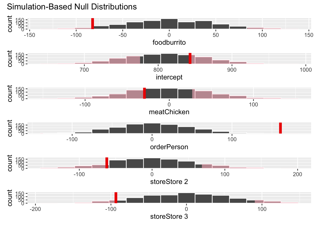
# bootstrap distribution for CIs
boot_full_dist <- chipotle |>
  specify(weight ~ order + meat + food + store) |>
  generate(reps = 1000, type = "bootstrap") |>
  fit()

# get 95% confidence interval
conf_ints <- get_ci(boot_full_dist, level = 0.95, point_estimate = obs_fit)

visualize(boot_full_dist) +
  shade_ci(endpoints = conf_ints)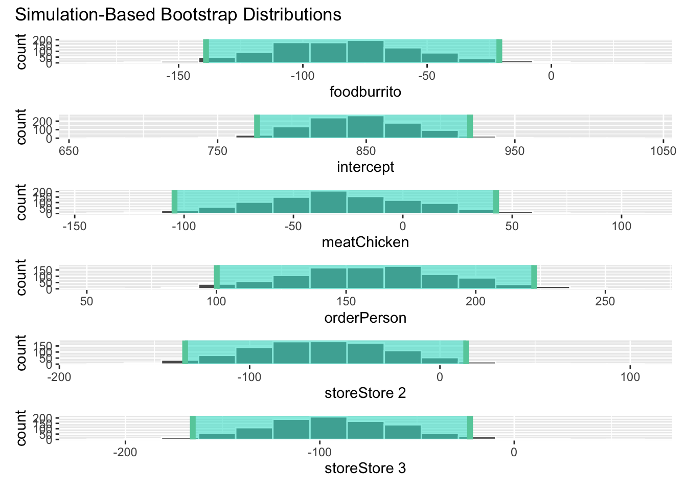
Please don’t. {infer} has several methods for visualizing \(p\)-values and confidence intervals, but they are best used for exploratory analysis, not for reporting results.
Do this instead
Once again, {gtsummary} can be used to create regression results tables.
# fit a standard linear regression model and rely on theoretical assumptions
# for confidence intervals and p-values
linear_reg() |>
  fit(weight ~ order + meat + food + store, data = chipotle) |>
  # basic results table
tbl_regression()| Characteristic | Beta | 95% CI | p-value |
|---|---|---|---|
| order | |||
| Online | — | — | |
| Person | 161 | 98, 223 | <0.001 |
| meat | |||
| Carnitas | — | — | |
| Chicken | -29 | -96, 38 | 0.4 |
| food | |||
| bowl | — | — | |
| burrito | -82 | -145, -20 | 0.012 |
| store | |||
| Store 1 | — | — | |
| Store 2 | -62 | -138, 14 | 0.10 |
| Store 3 | -93 | -169, -18 | 0.018 |
| Abbreviation: CI = Confidence Interval | |||
```{r}
#| tbl-cap: An example regression results table
linear_reg() |>
  fit(weight ~ order + meat + food + store, data = chipotle) |>
  # basic results table
  tbl_regression(
    # format variable labels
    label = list(
      order = "Order method",
      meat = "Meat",
      store = "Store",
      food = "Meal type"
    ),
    # round p-values to 2 significant digits
    pvalue_fun = label_style_pvalue(digits = 2)
    ) |>
  # add standard error and test statistic
  modify_header(
    statistic = "**Statistic**",
    std.error = "**SE**"
  ) |>
  # anything below the alpha threshold of 0.05 - format in bold
  bold_p(t = 0.05) |>
  # make labels bold
  bold_labels() |>
  # italicize levels for categorical variables
  italicize_levels()
```| Characteristic | Beta | SE | Statistic | 95% CI | p-value |
|---|---|---|---|---|---|
| Order method | |||||
| Online | — | — | — | — | |
| Person | 161 | 30.2 | 5.31 | 98, 223 | <0.001 |
| Meat | |||||
| Carnitas | — | — | — | — | |
| Chicken | -29 | 32.5 | -0.907 | -96, 38 | 0.37 |
| Meal type | |||||
| bowl | — | — | — | — | |
| burrito | -82 | 30.2 | -2.73 | -145, -20 | 0.012 |
| Store | |||||
| Store 1 | — | — | — | — | |
| Store 2 | -62 | 36.7 | -1.69 | -138, 14 | 0.10 |
| Store 3 | -93 | 36.7 | -2.54 | -169, -18 | 0.018 |
| Abbreviations: CI = Confidence Interval, SE = Standard Error | |||||
Use the tbl-cap code chunk option to add captions for tables produced programmatically. See the Quarto documentation for more examples of formatting tables using Quarto.
Alternatively, you can create a regression results plot that reports your estimated coefficients and CIs using a point range plot.
# visualize regression results using a coefficient plot
obs_fit |>
  # join with confidence intervals
  left_join(conf_ints) |>
  # order the coefficients by size, pull intercept to the beginning (by convention)
  mutate(term = fct_reorder(.f = term, .x = estimate) |>
    fct_relevel("intercept")) |>
  # draw a pointrange plot
  ggplot(mapping = aes(x = estimate, y = term, xmin = lower_ci, xmax = upper_ci)) +
  geom_pointrange() +
  # draw a vertical line at 0
  geom_vline(xintercept = 0, linetype = "dashed") +
  theme_minimal()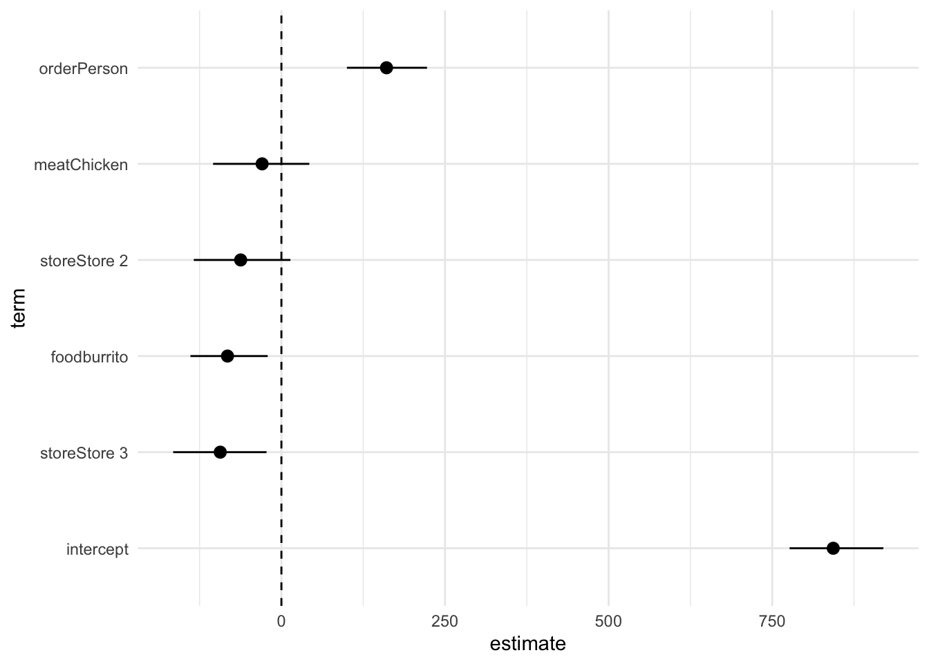
Notice this still requires substantial cleaning to make it publication-ready (e.g. title, axis labels, human-readable labels for each coefficient, etc.).
sessioninfo::session_info()─ Session info ───────────────────────────────────────────────────────────────
setting value
version R version 4.5.2 (2025-10-31)
os macOS Tahoe 26.3.1
system aarch64, darwin20
ui X11
language (EN)
collate en_US.UTF-8
ctype en_US.UTF-8
tz America/New_York
date 2026-03-13
pandoc 3.6.3 @ /Applications/Positron.app/Contents/Resources/app/quarto/bin/tools/aarch64/ (via rmarkdown)
quarto 1.9.33 @ /Applications/quarto/bin/quarto
─ Packages ───────────────────────────────────────────────────────────────────
! package * version date (UTC) lib source
P archive 1.1.12.1 2025-12-24 [?] RSPM
P backports 1.5.0 2024-05-23 [?] RSPM (R 4.5.0)
P base64enc 0.1-3 2015-07-28 [?] RSPM (R 4.5.0)
P bit 4.6.0 2025-03-06 [?] RSPM (R 4.5.0)
P bit64 4.6.0-1 2025-01-16 [?] RSPM (R 4.5.0)
P broom * 1.0.11 2025-12-04 [?] RSPM (R 4.5.0)
P broom.helpers 1.22.0 2025-09-17 [?] RSPM
P cards 0.7.1 2025-12-02 [?] CRAN (R 4.5.2)
P class 7.3-23 2025-01-01 [?] RSPM (R 4.5.0)
P cli 3.6.5 2025-04-23 [?] RSPM (R 4.5.0)
P codetools 0.2-20 2024-03-31 [?] RSPM (R 4.5.0)
P commonmark 2.0.0 2025-07-07 [?] RSPM (R 4.5.0)
P crayon 1.5.3 2024-06-20 [?] RSPM (R 4.5.0)
P data.table 1.18.0 2025-12-24 [?] RSPM (R 4.5.0)
P dials * 1.4.2 2025-09-04 [?] RSPM
P DiceDesign 1.10 2023-12-07 [?] RSPM (R 4.5.0)
P digest 0.6.39 2025-11-19 [?] RSPM (R 4.5.0)
P dplyr * 1.1.4 2023-11-17 [?] RSPM (R 4.5.0)
P evaluate 1.0.5 2025-08-27 [?] RSPM (R 4.5.0)
P farver 2.1.2 2024-05-13 [?] RSPM (R 4.5.0)
P fastmap 1.2.0 2024-05-15 [?] RSPM (R 4.5.0)
P forcats * 1.0.1 2025-09-25 [?] RSPM (R 4.5.0)
P fs 1.6.6 2025-04-12 [?] RSPM (R 4.5.0)
P furrr 0.3.1 2022-08-15 [?] RSPM
P future 1.68.0 2025-11-17 [?] RSPM
P future.apply 1.20.1 2025-12-09 [?] CRAN (R 4.5.2)
P generics 0.1.4 2025-05-09 [?] RSPM (R 4.5.0)
P ggplot2 * 4.0.1 2025-11-14 [?] RSPM (R 4.5.0)
P globals 0.18.0 2025-05-08 [?] RSPM
P glue 1.8.0 2024-09-30 [?] RSPM (R 4.5.0)
P gower 1.0.2 2024-12-17 [?] RSPM
P GPfit 1.0-9 2025-04-12 [?] RSPM (R 4.5.0)
P gt * 1.2.0 2025-12-16 [?] CRAN (R 4.5.2)
P gtable 0.3.6 2024-10-25 [?] RSPM (R 4.5.0)
P gtsummary * 2.5.0 2025-12-05 [?] CRAN (R 4.5.2)
P hardhat 1.4.2 2025-08-20 [?] RSPM
P haven 2.5.5 2025-05-30 [?] RSPM (R 4.5.0)
P here 1.0.2 2025-09-15 [?] CRAN (R 4.5.0)
P hms 1.1.4 2025-10-17 [?] RSPM (R 4.5.0)
P htmltools 0.5.9 2025-12-04 [?] RSPM (R 4.5.0)
P htmlwidgets 1.6.4 2023-12-06 [?] RSPM (R 4.5.0)
P infer * 1.1.0 2025-12-18 [?] CRAN (R 4.5.2)
P ipred 0.9-15 2024-07-18 [?] RSPM
P jsonlite 2.0.0 2025-03-27 [?] RSPM (R 4.5.0)
P knitr 1.51 2025-12-20 [?] RSPM (R 4.5.0)
P labeling 0.4.3 2023-08-29 [?] RSPM (R 4.5.0)
P labelled 2.16.0 2025-10-22 [?] RSPM
P lattice 0.22-7 2025-04-02 [?] RSPM (R 4.5.0)
P lava 1.8.2 2025-10-30 [?] RSPM
P lhs 1.2.0 2024-06-30 [?] RSPM (R 4.5.0)
P lifecycle 1.0.4 2023-11-07 [?] RSPM (R 4.5.0)
P listenv 0.10.0 2025-11-02 [?] RSPM
P litedown 0.9 2025-12-18 [?] CRAN (R 4.5.2)
P lubridate * 1.9.4 2024-12-08 [?] RSPM (R 4.5.0)
P magrittr 2.0.4 2025-09-12 [?] RSPM (R 4.5.0)
P markdown 2.0 2025-03-23 [?] RSPM (R 4.5.0)
P MASS 7.3-65 2025-02-28 [?] RSPM (R 4.5.0)
P Matrix 1.7-4 2025-08-28 [?] RSPM (R 4.5.0)
P modeldata * 1.5.1 2025-08-22 [?] RSPM
P nnet 7.3-20 2025-01-01 [?] RSPM (R 4.5.0)
P otel 0.2.0 2025-08-29 [?] RSPM (R 4.5.0)
P parallelly 1.46.0 2025-12-12 [?] CRAN (R 4.5.2)
P parsnip * 1.4.0 2025-12-01 [?] CRAN (R 4.5.2)
P pillar 1.11.1 2025-09-17 [?] RSPM (R 4.5.0)
P pkgconfig 2.0.3 2019-09-22 [?] RSPM (R 4.5.0)
P prodlim 2025.04.28 2025-04-28 [?] RSPM
P purrr * 1.2.0 2025-11-04 [?] CRAN (R 4.5.0)
P R6 2.6.1 2025-02-15 [?] RSPM (R 4.5.0)
P RColorBrewer 1.1-3 2022-04-03 [?] RSPM (R 4.5.0)
P Rcpp 1.1.0 2025-07-02 [?] RSPM (R 4.5.0)
P readr * 2.1.6 2025-11-14 [?] RSPM (R 4.5.0)
P recipes * 1.3.1 2025-05-21 [?] RSPM
renv 1.1.5 2025-07-24 [1] RSPM (R 4.5.0)
P repr 1.1.7 2024-03-22 [?] RSPM
P rlang 1.1.6 2025-04-11 [?] RSPM (R 4.5.0)
P rmarkdown 2.30 2025-09-28 [?] RSPM (R 4.5.0)
P rpart 4.1.24 2025-01-07 [?] RSPM (R 4.5.0)
P rprojroot 2.1.1 2025-08-26 [?] RSPM (R 4.5.0)
P rsample * 1.3.1 2025-07-29 [?] RSPM
P rstudioapi 0.17.1 2024-10-22 [?] RSPM (R 4.5.0)
P S7 0.2.1 2025-11-14 [?] RSPM (R 4.5.0)
P sass 0.4.10 2025-04-11 [?] RSPM (R 4.5.0)
P scales * 1.4.0 2025-04-24 [?] RSPM (R 4.5.0)
P sessioninfo 1.2.3 2025-02-05 [?] RSPM (R 4.5.0)
P skimr * 2.2.1 2025-07-26 [?] RSPM
P sparsevctrs 0.3.5 2025-12-09 [?] CRAN (R 4.5.2)
P stringi 1.8.7 2025-03-27 [?] RSPM (R 4.5.0)
P stringr * 1.6.0 2025-11-04 [?] RSPM (R 4.5.0)
P survival 3.8-3 2024-12-17 [?] RSPM (R 4.5.0)
P tailor * 0.1.0 2025-08-25 [?] RSPM
P tibble * 3.3.0 2025-06-08 [?] RSPM (R 4.5.0)
P tidymodels * 1.4.1 2025-09-08 [?] RSPM
P tidyr * 1.3.2 2025-12-19 [?] RSPM (R 4.5.0)
P tidyselect 1.2.1 2024-03-11 [?] RSPM (R 4.5.0)
P tidyverse * 2.0.0 2023-02-22 [?] RSPM (R 4.5.0)
P timechange 0.3.0 2024-01-18 [?] RSPM (R 4.5.0)
P timeDate 4051.111 2025-10-17 [?] RSPM
P tune * 2.0.1 2025-10-17 [?] RSPM
P tzdb 0.5.0 2025-03-15 [?] RSPM (R 4.5.0)
P vctrs 0.6.5 2023-12-01 [?] RSPM (R 4.5.0)
P vroom 1.6.7 2025-11-28 [?] RSPM (R 4.5.0)
P withr 3.0.2 2024-10-28 [?] RSPM (R 4.5.0)
P workflows * 1.3.0 2025-08-27 [?] RSPM
P workflowsets * 1.1.1 2025-05-27 [?] RSPM
P xfun 0.55 2025-12-16 [?] CRAN (R 4.5.2)
P xml2 1.5.1 2025-12-01 [?] RSPM
P yaml 2.3.12 2025-12-10 [?] RSPM (R 4.5.0)
P yardstick * 1.3.2 2025-01-22 [?] RSPM
[1] /Users/bcs88/Projects/info-2950/course-site/renv/library/macos/R-4.5/aarch64-apple-darwin20
[2] /Users/bcs88/Library/Caches/org.R-project.R/R/renv/sandbox/macos/R-4.5/aarch64-apple-darwin20/4cd76b74
* ── Packages attached to the search path.
P ── Loaded and on-disk path mismatch.
──────────────────────────────────────────────────────────────────────────────