AE 25: Slay – Predicting song artist based on lyrics

Suggested answers

library(tidyverse)
library(tidymodels)
library(stringr)
library(textrecipes)
library(textdata)
library(discrim)
library(themis)
library(vip)

# set seed for randomization
set.seed(123)

theme_set(theme_minimal())

Import data

lyrics <- read_csv(file = "data/beyonce-swift-lyrics.csv") |>
  mutate(artist = factor(artist))
lyrics

# A tibble: 355 × 19
   album_name track_number track_name artist lyrics danceability energy loudness
   <chr>             <dbl> <chr>      <fct>  <chr>         <dbl>  <dbl>    <dbl>
 1 COWBOY CA…            1 AMERIICAN… Beyon… "Noth…        0.374  0.515    -6.48
 2 COWBOY CA…            3 16 CARRIA… Beyon… "Sixt…        0.525  0.456    -7.04
 3 COWBOY CA…            5 MY ROSE    Beyon… "How …        0.384  0.177   -11.8 
 4 COWBOY CA…            7 TEXAS HOL… Beyon… "This…        0.727  0.711    -6.55
 5 COWBOY CA…            8 BODYGUARD  Beyon… "One,…        0.726  0.779    -5.43
 6 COWBOY CA…           10 JOLENE     Beyon… "(Jol…        0.567  0.812    -5.43
 7 COWBOY CA…           11 DAUGHTER   Beyon… "Your…        0.374  0.448   -10.0 
 8 COWBOY CA…           13 ALLIIGATO… Beyon… "High…        0.618  0.651    -9.66
 9 COWBOY CA…           18 FLAMENCO   Beyon… "My m…        0.497  0.351    -9.25
10 COWBOY CA…           20 YA YA      Beyon… "Hell…        0.617  0.904    -5.37
# ℹ 345 more rows
# ℹ 11 more variables: speechiness <dbl>, acousticness <dbl>,
#   instrumentalness <dbl>, liveness <dbl>, valence <dbl>, tempo <dbl>,
#   time_signature <dbl>, duration_ms <dbl>, explicit <lgl>, key_name <chr>,
#   mode_name <chr>

Split the data into analysis/assessment/test sets

Demonstration:

• Split the data into training/test sets with 75% allocated for training
• Split the training set into 10 cross-validation folds

# split into training/testing
set.seed(123)
lyrics_split <- initial_split(data = lyrics, strata = artist, prop = 0.75)

lyrics_train <- training(lyrics_split)
lyrics_test <- testing(lyrics_split)

# create cross-validation folds
lyrics_folds <- vfold_cv(data = lyrics_train, strata = artist)

Estimate the null model for a baseline comparison

Demonstration: Estimate a null model to determine an appropriate baseline for evaluating a model’s performance.

null_spec <- null_model() |>
  set_engine("parsnip") |>
  set_mode("classification")

null_spec |>
  fit_resamples(
    # pick something as the predictor - doesn't really matter
    artist ~ danceability,
    resamples = lyrics_folds
  ) |>
  collect_metrics()

# A tibble: 3 × 6
  .metric     .estimator  mean     n  std_err .config             
  <chr>       <chr>      <dbl> <int>    <dbl> <chr>               
1 accuracy    binary     0.668    10 0.00236  Preprocessor1_Model1
2 brier_class binary     0.222    10 0.000792 Preprocessor1_Model1
3 roc_auc     binary     0.5      10 0        Preprocessor1_Model1

Fit a random forest model

Define the feature engineering recipe

Demonstration:

• Define a feature engineering recipe to predict the song’s artist as a function of the lyrics + audio features
• Exclude the ID variables from the recipe
• Tokenize the song lyrics
• Remove stop words
• Only keep the 500 most frequently appearing tokens
• Calculate tf-idf scores for the remaining tokens
• Downsample the observations so there are an equal number of songs by Beyoncé and Taylor Swift in the analysis set

# define preprocessing recipe
rf_rec <- recipe(artist ~ ., data = lyrics_train) |>
  # exclude ID variables
  update_role(album_name, track_number, track_name, new_role = "id vars") |>
  step_tokenize(lyrics) |>
  step_stopwords(lyrics) |>
  step_tokenfilter(lyrics, max_tokens = 500) |>
  step_tfidf(lyrics) |>
  step_downsample(artist)
rf_rec

Fit the model

Demonstration:

• Define a random forest model grown with 1000 trees using the ranger engine.
• Define a workflow using the feature engineering recipe and random forest model specification. Fit the workflow using the cross-validation folds.
  • Use control = control_resamples(save_pred = TRUE) to save the assessment set predictions. We need these to assess the model’s performance.
  • Use control = control_resamples(save_workflow = TRUE) to save the workflow object. We need this later on if we want to fit a single model using the same workflow and the entire training set.

# define the model specification
rf_spec <- rand_forest(trees = 1000) |>
  set_mode("classification") |>
  # calculate feature importance metrics using the ranger engine
  set_engine("ranger", importance = "permutation")

# define the workflow
rf_wf <- workflow() |>
  add_recipe(rf_rec) |>
  add_model(rf_spec)

# fit the model to each of the cross-validation folds
rf_cv <- rf_wf |>
  fit_resamples(
    resamples = lyrics_folds,
    control = control_resamples(save_pred = TRUE, save_workflow = TRUE)
  )

Evaluate model performance

Demonstration:

• Calculate the model’s accuracy and ROC AUC. How did it perform?
• Draw the ROC curve for each validation fold
• Generate the resampled confusion matrix for the model and draw it using a heatmap. How does the model perform predicting Beyoncé songs relative to Taylor Swift songs?

# extract metrics and predictions
rf_cv_metrics <- collect_metrics(rf_cv)
rf_cv_predictions <- collect_predictions(rf_cv)

# how well did the model perform?
rf_cv_metrics

# A tibble: 3 × 6
  .metric     .estimator  mean     n std_err .config             
  <chr>       <chr>      <dbl> <int>   <dbl> <chr>               
1 accuracy    binary     0.872    10 0.0256  Preprocessor1_Model1
2 brier_class binary     0.156    10 0.00544 Preprocessor1_Model1
3 roc_auc     binary     0.920    10 0.0195  Preprocessor1_Model1

# roc curve
rf_cv_predictions |>
  group_by(id) |>
  roc_curve(truth = artist, .pred_Beyoncé) |>
  autoplot()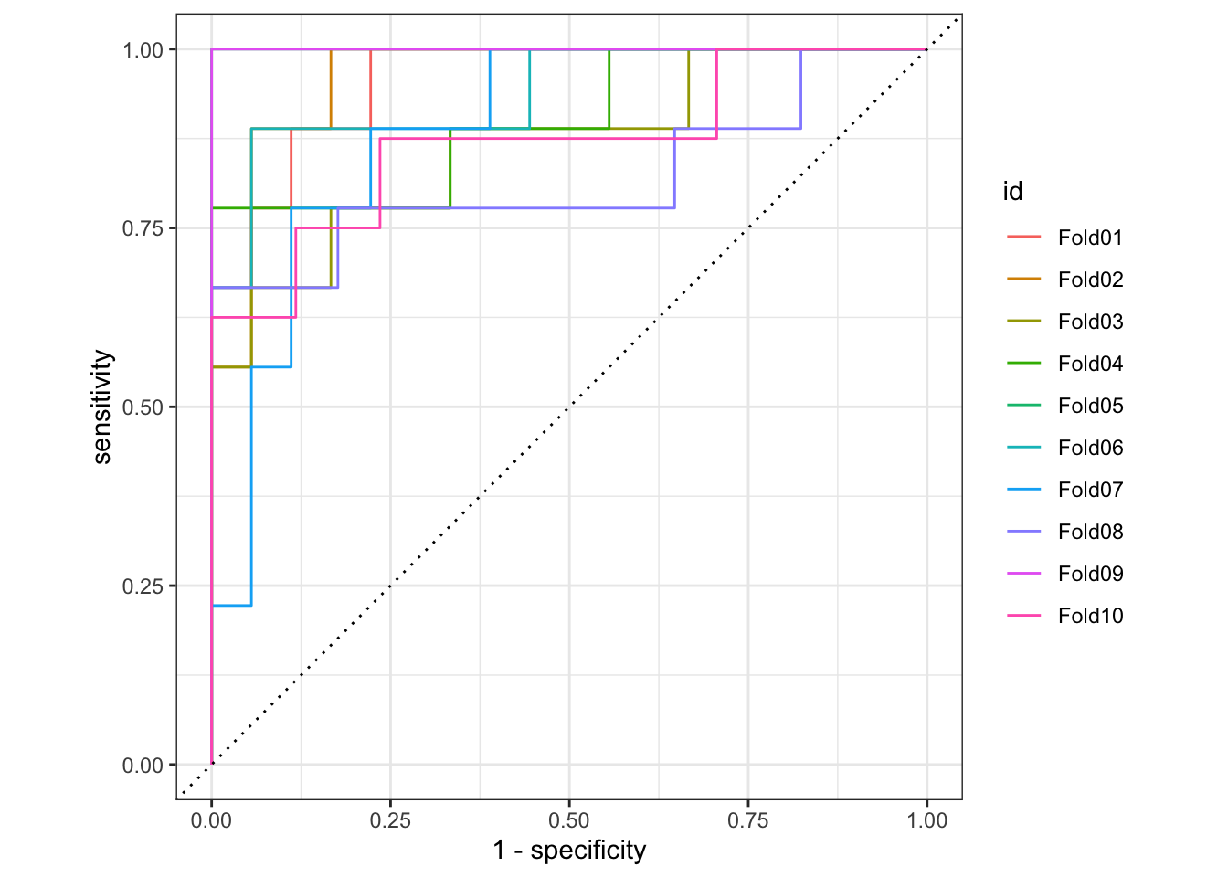

# confusion matrix
conf_mat_resampled(x = rf_cv, tidy = FALSE) |>
  autoplot(type = "heatmap")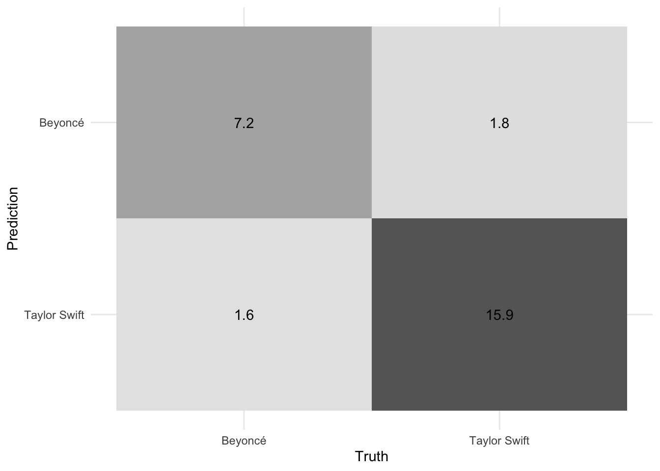

Add response here. Overall this is a pretty strong model. The ROC AUC is quite strong. The confusion matrix shows that the model is slightly better at predicting Taylor Swift songs than Beyoncé songs, but given the overrepresentation of Taylor Swift songs in the dataset this is not unusual.

Penalized regression

Define the feature engineering recipe

Demonstration:

• Define a feature engineering recipe to predict the song’s artist as a function of the lyrics + audio features
• Exclude the ID variables from the recipe
• Tokenize the song lyrics
• Calculate all possible 1-grams, 2-grams, 3-grams, 4-grams, and 5-grams
• Remove stop words
• Only keep the 2000 most frequently appearing tokens
• Calculate tf-idf scores for the remaining tokens
• Apply required steps for penalized regression models
  • Convert the explicit variable to a factor
  • Convert nominal predictors to dummy variables
  • Get rid of zero-variance predictors
  • Normalize all predictors to mean of 0 and variance of 1
• Downsample the observations so there are an equal number of songs by Beyoncé and Taylor Swift in the analysis set

glmnet_rec <- recipe(artist ~ ., data = lyrics_train) |>
  # exclude ID variables
  update_role(album_name, track_number, track_name, new_role = "id vars") |>
  # tokenize and prep lyrics
  step_tokenize(lyrics) |>
  step_stopwords(lyrics) |>
  step_ngram(lyrics, num_tokens = 5L, min_num_tokens = 1L) |>
  step_tokenfilter(lyrics, max_tokens = 2000) |>
  step_tfidf(lyrics) |>
  # fix explicit variable to factor
  step_bin2factor(explicit) |>
  # normalize for penalized regression
  step_dummy(all_nominal_predictors()) |>
  step_zv(all_predictors()) |>
  step_normalize(all_numeric_predictors()) |>
  step_downsample(artist)
glmnet_rec

Tune the penalized regression model

Demonstration:

• Define the penalized regression model specification, including tuning placeholders for penalty and mixture
• Create the workflow object
• Define a tuning grid with every combination of:
  • penalty = 10^seq(-6, -1, length.out = 20)
  • mixture = c(0, 0.2, 0.4, 0.6, 0.8, 1)
• Tune the model using the cross-validation folds
• Evaluate the tuning procedure and identify the best performing models based on ROC AUC

# define the penalized regression model specification
glmnet_spec <- logistic_reg(penalty = tune(), mixture = tune()) |>
  set_mode("classification") |>
  set_engine("glmnet")

# define the new workflow
glmnet_wf <- workflow() |>
  add_recipe(glmnet_rec) |>
  add_model(glmnet_spec)

# create the tuning grid
glmnet_grid <- expand_grid(
  penalty = 10^seq(-6, -1, length.out = 20),
  mixture = c(0, 0.2, 0.4, 0.6, 0.8, 1)
)

# tune over the model hyperparameters
glmnet_tune <- tune_grid(
  object = glmnet_wf,
  resamples = lyrics_folds,
  grid = glmnet_grid,
  control = control_grid(save_pred = TRUE, save_workflow = TRUE)
)

# evaluate results
collect_metrics(x = glmnet_tune)

# A tibble: 360 × 8
      penalty mixture .metric     .estimator  mean     n std_err .config        
        <dbl>   <dbl> <chr>       <chr>      <dbl> <int>   <dbl> <chr>          
 1 0.000001         0 accuracy    binary     0.818    10 0.0203  Preprocessor1_…
 2 0.000001         0 brier_class binary     0.160    10 0.00516 Preprocessor1_…
 3 0.000001         0 roc_auc     binary     0.891    10 0.0176  Preprocessor1_…
 4 0.00000183       0 accuracy    binary     0.818    10 0.0203  Preprocessor1_…
 5 0.00000183       0 brier_class binary     0.160    10 0.00516 Preprocessor1_…
 6 0.00000183       0 roc_auc     binary     0.891    10 0.0176  Preprocessor1_…
 7 0.00000336       0 accuracy    binary     0.818    10 0.0203  Preprocessor1_…
 8 0.00000336       0 brier_class binary     0.160    10 0.00516 Preprocessor1_…
 9 0.00000336       0 roc_auc     binary     0.891    10 0.0176  Preprocessor1_…
10 0.00000616       0 accuracy    binary     0.818    10 0.0203  Preprocessor1_…
# ℹ 350 more rows

autoplot(glmnet_tune)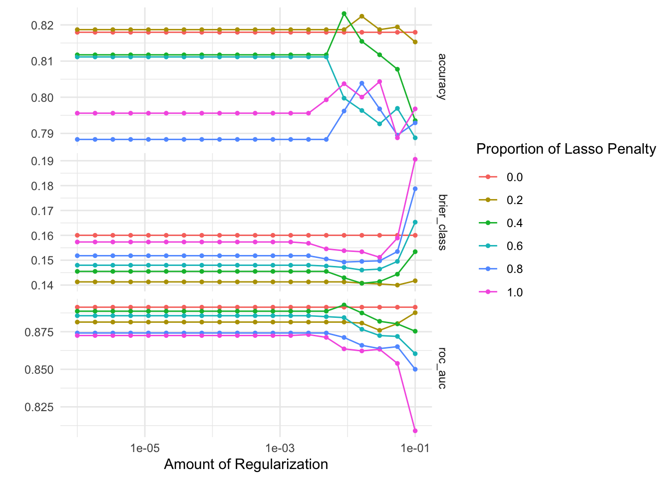

# identify the five best hyperparameter combinations
show_best(x = glmnet_tune, metric = "roc_auc")

# A tibble: 5 × 8
     penalty mixture .metric .estimator  mean     n std_err .config             
       <dbl>   <dbl> <chr>   <chr>      <dbl> <int>   <dbl> <chr>               
1 0.00886        0.4 roc_auc binary     0.893    10  0.0194 Preprocessor1_Model…
2 0.000001       0   roc_auc binary     0.891    10  0.0176 Preprocessor1_Model…
3 0.00000183     0   roc_auc binary     0.891    10  0.0176 Preprocessor1_Model…
4 0.00000336     0   roc_auc binary     0.891    10  0.0176 Preprocessor1_Model…
5 0.00000616     0   roc_auc binary     0.891    10  0.0176 Preprocessor1_Model…

Add response here. The best performing hyperparameter combination has a strong ROC AUC value, though it is slightly lower compared to the random forest model.

Random forest with word embeddings

Define the feature engineering recipe

Demonstration: Rather than using individual tokens and tf-idf scores, we will use pre-trained word embeddings to represent the lyrics. We will calculate the aggregate embedding for each song by averaging the embeddings of all the words in the song, then tune a random forest model using these embeddings.

Importing GloVe embeddings

Normally in order to import GloVe embeddings you would use the code below:

glove_embed <- embedding_glove6b(dimensions = 100)

This downloads the ZIP file containing the embeddings, stores it in a cache folder, and then imports the requested embeddings and dimensions as a data frame. Note that many of the embeddings are stored in ZIP files that are multiple gigabytes in size. Often it is easier to manually download the files and store them in the appropriate location outside of R. See the documentation for embedding_glove*() for more information.

# hacky way to make it work on RStudio Workbench
glove_embed <- read_delim(
    file = "/rstudio-files/glove6b/glove.6B.100d.txt",
    delim = " ",
    quote = "",
    col_names = c(
      "token",
      paste0("d", seq_len(100))
    ),
    col_types = paste0(
      c(
        "c",
        rep("d", 100)
      ),
      collapse = ""
    )
  )

# load previously-downloaded word embeddings
glove_embed <- embedding_glove6b(
  # dir = "/rstudio-files",
  dimensions = 100,
  manual_download = TRUE
)

rf_embeds_rec <- recipe(artist ~ ., data = lyrics_train) |>
  # exclude ID variables
  update_role(album_name, track_number, track_name, new_role = "id vars") |>
  step_tokenize(lyrics) |>
  # calculate aggregate embedding for each song
  step_word_embeddings(lyrics, embeddings = glove_embed, aggregation = "mean") |>
  step_downsample(artist)
rf_embeds_rec

Tune the model

Demonstration:

• Define the penalized regression model specification, including tuning placeholders for mtry and min_n
• Create the workflow object
• Tune the model using the cross-validation folds and an automatically generated tuning grid
• Evaluate the tuning procedure and identify the best performing models based on ROC AUC

# define the model specification
rf_embeds_spec <- rand_forest(trees = 1000, mtry = tune(), min_n = tune()) |>
  set_mode("classification") |>
  # calculate feature importance metrics using the ranger engine
  set_engine("ranger", importance = "permutation")

# define the workflow
rf_embeds_wf <- workflow() |>
  add_recipe(rf_embeds_rec) |>
  add_model(rf_embeds_spec)

# fit the model to each of the cross-validation folds
rf_embeds_cv <- rf_embeds_wf |>
  tune_grid(
    resamples = lyrics_folds,
    control = control_resamples(save_pred = TRUE, save_workflow = TRUE)
  )

# extract metrics
rf_embeds_cv_metrics <- collect_metrics(rf_embeds_cv)

# how well did the model perform?
rf_embeds_cv_metrics

# A tibble: 30 × 8
    mtry min_n .metric     .estimator  mean     n std_err .config              
   <int> <int> <chr>       <chr>      <dbl> <int>   <dbl> <chr>                
 1    75    26 accuracy    binary     0.820    10  0.0320 Preprocessor1_Model01
 2    75    26 brier_class binary     0.152    10  0.0118 Preprocessor1_Model01
 3    75    26 roc_auc     binary     0.872    10  0.0294 Preprocessor1_Model01
 4    99     7 accuracy    binary     0.823    10  0.0331 Preprocessor1_Model02
 5    99     7 brier_class binary     0.148    10  0.0119 Preprocessor1_Model02
 6    99     7 roc_auc     binary     0.882    10  0.0279 Preprocessor1_Model02
 7    61    39 accuracy    binary     0.827    10  0.0284 Preprocessor1_Model03
 8    61    39 brier_class binary     0.153    10  0.0111 Preprocessor1_Model03
 9    61    39 roc_auc     binary     0.875    10  0.0282 Preprocessor1_Model03
10    14    23 accuracy    binary     0.816    10  0.0295 Preprocessor1_Model04
# ℹ 20 more rows

show_best(rf_embeds_cv, metric = "roc_auc")

# A tibble: 5 × 8
   mtry min_n .metric .estimator  mean     n std_err .config              
  <int> <int> <chr>   <chr>      <dbl> <int>   <dbl> <chr>                
1    32     4 roc_auc binary     0.888    10  0.0236 Preprocessor1_Model05
2    99     7 roc_auc binary     0.882    10  0.0279 Preprocessor1_Model02
3    39    17 roc_auc binary     0.881    10  0.0270 Preprocessor1_Model06
4    55    30 roc_auc binary     0.877    10  0.0284 Preprocessor1_Model09
5    61    39 roc_auc binary     0.875    10  0.0282 Preprocessor1_Model03

Add response here. The random forest model using word embeddings performed better than the penalized regression model, but not as well as the random forest model using tf-idf scores. That said, all the ROC AUC values are quite close to each other.

Fit the best model

Your turn:

• Select the model + hyperparameter combinations that achieve the highest ROC AUC
• Fit that model using the best hyperparameters and the full training set. How well does the model perform on the test set?

# select the best model's hyperparameters
best_fit <- fit_best(rf_cv)

# test set ROC AUC
augment(best_fit, new_data = lyrics_test) |>
  roc_auc(truth = artist, .pred_Beyoncé)

# A tibble: 1 × 3
  .metric .estimator .estimate
  <chr>   <chr>          <dbl>
1 roc_auc binary         0.939

Add response here. The test set ROC AUC is slightly higher than the cross-validated metrics, indicating that the model generalizes well to new data.

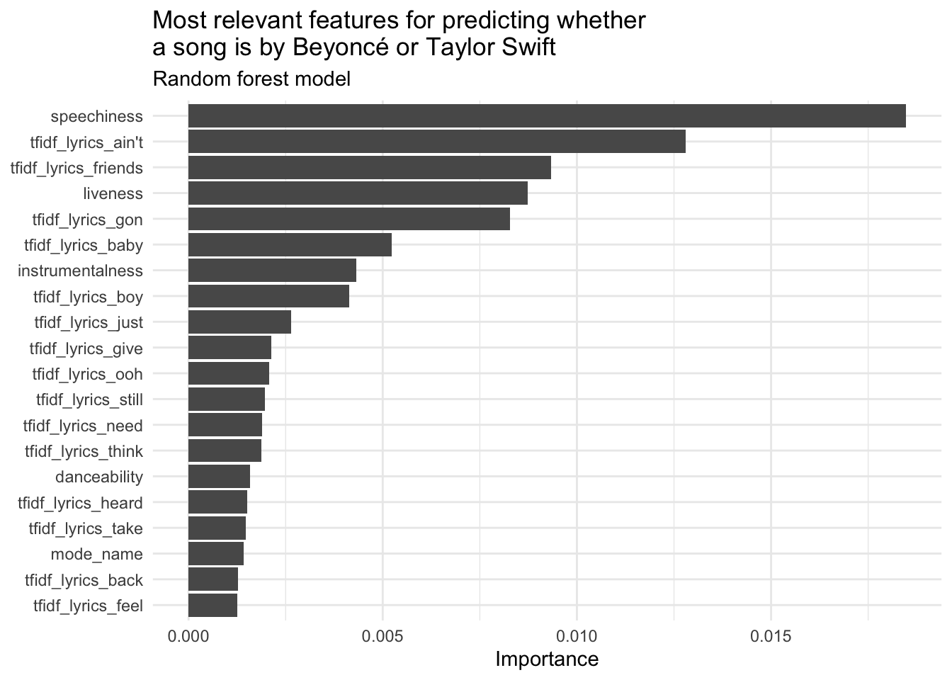
Variable importance

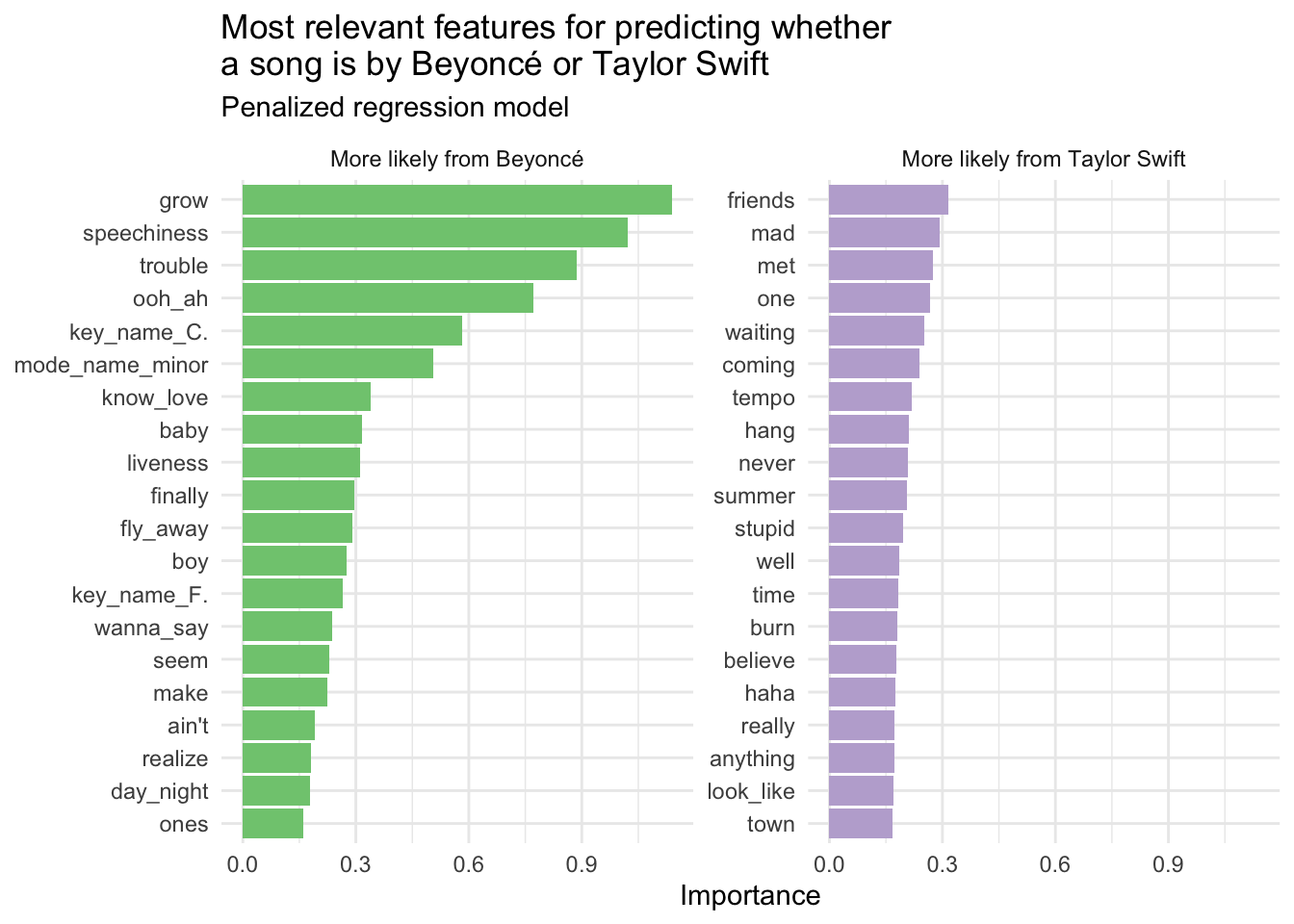
We can examine the results of each model to evaluate which tokens were the most important in generating artist predictions. Here we use {vip} to calculate importance.

# extract parsnip model fit
rf_imp <- rf_cv |>
  fit_best() |>
  extract_fit_parsnip() |>
  vi(method = "model")

# clean up the data frame for visualization
rf_imp |>
  # extract 20 most important n-grams
  slice_max(order_by = Importance, n = 20) |>
  mutate(Variable = fct_reorder(.f = Variable, .x = Importance)) |>
  ggplot(mapping = aes(
    x = Importance,
    y = Variable
  )) +
  geom_col() +
  labs(
    y = NULL,
    title = "Most relevant features for predicting whether\na song is by Beyoncé or Taylor Swift",
    subtitle = "Random forest model"
  )

# extract parsnip model fit
glmnet_imp <- glmnet_tune |>
  fit_best() |>
  extract_fit_parsnip() |>
  vi(method = "model", lambda = select_best(x = glmnet_tune, metric = "roc_auc")$penalty)

# clean up the data frame for visualization
glmnet_imp |>
  mutate(
    Sign = case_when(
      Sign == "NEG" ~ "More likely from Beyoncé",
      Sign == "POS" ~ "More likely from Taylor Swift"
    ),
    Importance = abs(Importance)
  ) |>
  # importance must be greater than 0
  filter(Importance > 0) |>
  # remove the "tfidf_lyrics_" prefix
  mutate(Variable = str_replace_all(string = Variable, pattern = "tfidf_lyrics_", replacement = "")) |>
  # keep top 20 features for each artist
  slice_max(n = 20, order_by = Importance, by = Sign) |>
  mutate(Variable = fct_reorder(.f = Variable, .x = Importance)) |>
  ggplot(mapping = aes(
    x = Importance,
    y = Variable,
    fill = Sign
  )) +
  geom_col(show.legend = FALSE) +
  scale_fill_brewer(type = "qual") +
  facet_wrap(facets = vars(Sign), scales = "free_y") +
  labs(
    y = NULL,
    title = "Most relevant features for predicting whether\na song is by Beyoncé or Taylor Swift",
    subtitle = "Penalized regression model"
  )

Session information

sessioninfo::session_info()

─ Session info ───────────────────────────────────────────────────────────────
 setting  value
 version  R version 4.4.2 (2024-10-31)
 os       macOS Sonoma 14.6.1
 system   aarch64, darwin20
 ui       X11
 language (EN)
 collate  en_US.UTF-8
 ctype    en_US.UTF-8
 tz       America/New_York
 date     2025-05-04
 pandoc   3.4 @ /usr/local/bin/ (via rmarkdown)

─ Packages ───────────────────────────────────────────────────────────────────
 package      * version    date (UTC) lib source
 archive        1.1.9      2024-09-12 [1] CRAN (R 4.4.1)
 backports      1.5.0      2024-05-23 [1] CRAN (R 4.4.0)
 bit            4.6.0      2025-03-06 [1] RSPM
 bit64          4.6.0-1    2025-01-16 [1] RSPM
 broom        * 1.0.8      2025-03-28 [1] CRAN (R 4.4.1)
 class          7.3-22     2023-05-03 [1] CRAN (R 4.4.2)
 cli            3.6.4      2025-02-13 [1] CRAN (R 4.4.1)
 codetools      0.2-20     2024-03-31 [1] CRAN (R 4.4.2)
 crayon         1.5.3      2024-06-20 [1] CRAN (R 4.4.0)
 data.table     1.17.0     2025-02-22 [1] RSPM
 dials        * 1.3.0      2024-07-30 [1] CRAN (R 4.4.0)
 DiceDesign     1.10       2023-12-07 [1] CRAN (R 4.3.1)
 dichromat      2.0-0.1    2022-05-02 [1] CRAN (R 4.3.0)
 digest         0.6.37     2024-08-19 [1] CRAN (R 4.4.1)
 discrim      * 1.0.1      2023-03-08 [1] CRAN (R 4.3.0)
 dplyr        * 1.1.4      2023-11-17 [1] CRAN (R 4.3.1)
 ellipsis       0.3.2      2021-04-29 [1] CRAN (R 4.3.0)
 evaluate       1.0.3      2025-01-10 [1] CRAN (R 4.4.1)
 farver         2.1.2      2024-05-13 [1] CRAN (R 4.3.3)
 fastmap        1.2.0      2024-05-15 [1] CRAN (R 4.4.0)
 forcats      * 1.0.0      2023-01-29 [1] CRAN (R 4.3.0)
 foreach        1.5.2      2022-02-02 [1] CRAN (R 4.3.0)
 fs             1.6.6      2025-04-12 [1] RSPM
 furrr          0.3.1      2022-08-15 [1] CRAN (R 4.3.0)
 future         1.33.2     2024-03-26 [1] CRAN (R 4.3.1)
 future.apply   1.11.2     2024-03-28 [1] CRAN (R 4.3.1)
 generics       0.1.3      2022-07-05 [1] CRAN (R 4.3.0)
 ggplot2      * 3.5.2      2025-04-09 [1] RSPM
 glmnet       * 4.1-8      2023-08-22 [1] CRAN (R 4.3.0)
 globals        0.16.3     2024-03-08 [1] CRAN (R 4.3.1)
 glue           1.8.0      2024-09-30 [1] CRAN (R 4.4.1)
 gower          1.0.1      2022-12-22 [1] CRAN (R 4.3.0)
 GPfit          1.0-8      2019-02-08 [1] CRAN (R 4.3.0)
 gtable         0.3.6      2024-10-25 [1] CRAN (R 4.4.1)
 hardhat        1.4.0      2024-06-02 [1] CRAN (R 4.4.0)
 here           1.0.1      2020-12-13 [1] CRAN (R 4.3.0)
 hms            1.1.3      2023-03-21 [1] CRAN (R 4.3.0)
 htmltools      0.5.8.1    2024-04-04 [1] CRAN (R 4.3.1)
 htmlwidgets    1.6.4      2023-12-06 [1] CRAN (R 4.3.1)
 infer        * 1.0.7      2024-03-25 [1] CRAN (R 4.3.1)
 ipred          0.9-14     2023-03-09 [1] CRAN (R 4.3.0)
 iterators      1.0.14     2022-02-05 [1] CRAN (R 4.3.0)
 jsonlite       2.0.0      2025-03-27 [1] RSPM
 knitr          1.50       2025-03-16 [1] CRAN (R 4.4.1)
 labeling       0.4.3      2023-08-29 [1] CRAN (R 4.3.0)
 lattice        0.22-6     2024-03-20 [1] CRAN (R 4.4.2)
 lava           1.8.0      2024-03-05 [1] CRAN (R 4.3.1)
 lhs            1.1.6      2022-12-17 [1] CRAN (R 4.3.0)
 lifecycle      1.0.4      2023-11-07 [1] CRAN (R 4.3.1)
 listenv        0.9.1      2024-01-29 [1] CRAN (R 4.3.1)
 lubridate    * 1.9.4      2024-12-08 [1] RSPM
 magrittr       2.0.3      2022-03-30 [1] CRAN (R 4.3.0)
 MASS           7.3-61     2024-06-13 [1] CRAN (R 4.4.2)
 Matrix       * 1.7-1      2024-10-18 [1] CRAN (R 4.4.2)
 modeldata    * 1.4.0      2024-06-19 [1] CRAN (R 4.4.0)
 modelenv       0.1.1      2023-03-08 [1] CRAN (R 4.3.0)
 nnet           7.3-19     2023-05-03 [1] CRAN (R 4.4.2)
 parallelly     1.37.1     2024-02-29 [1] CRAN (R 4.3.1)
 parsnip      * 1.2.1      2024-03-22 [1] CRAN (R 4.3.1)
 pillar         1.10.2     2025-04-05 [1] CRAN (R 4.4.1)
 pkgconfig      2.0.3      2019-09-22 [1] CRAN (R 4.3.0)
 prodlim        2023.08.28 2023-08-28 [1] CRAN (R 4.3.0)
 purrr        * 1.0.4      2025-02-05 [1] RSPM
 R6             2.6.1      2025-02-15 [1] RSPM
 ranger       * 0.16.0     2023-11-12 [1] CRAN (R 4.3.1)
 rappdirs       0.3.3      2021-01-31 [1] CRAN (R 4.3.0)
 RColorBrewer   1.1-3      2022-04-03 [1] CRAN (R 4.3.0)
 Rcpp           1.0.14     2025-01-12 [1] CRAN (R 4.4.1)
 readr        * 2.1.5      2024-01-10 [1] CRAN (R 4.3.1)
 recipes      * 1.0.10     2024-02-18 [1] CRAN (R 4.3.1)
 rlang          1.1.6      2025-04-11 [1] RSPM
 rmarkdown      2.29       2024-11-04 [1] CRAN (R 4.4.1)
 ROSE           0.0-4      2021-06-14 [1] CRAN (R 4.3.0)
 rpart          4.1.23     2023-12-05 [1] CRAN (R 4.4.2)
 rprojroot      2.0.4      2023-11-05 [1] CRAN (R 4.3.1)
 rsample      * 1.2.1      2024-03-25 [1] CRAN (R 4.3.1)
 rstudioapi     0.17.1     2024-10-22 [1] RSPM
 scales       * 1.4.0      2025-04-24 [1] CRAN (R 4.4.1)
 sessioninfo    1.2.2      2021-12-06 [1] CRAN (R 4.3.0)
 shape          1.4.6.1    2024-02-23 [1] CRAN (R 4.3.1)
 SnowballC      0.7.1      2023-04-25 [1] CRAN (R 4.3.0)
 stopwords    * 2.3        2021-10-28 [1] CRAN (R 4.3.0)
 stringi        1.8.7      2025-03-27 [1] RSPM
 stringr      * 1.5.1      2023-11-14 [1] CRAN (R 4.3.1)
 survival       3.7-0      2024-06-05 [1] CRAN (R 4.4.2)
 textdata     * 0.4.5      2024-05-28 [1] CRAN (R 4.4.0)
 textrecipes  * 1.0.6      2023-11-15 [1] CRAN (R 4.3.1)
 themis       * 1.0.2      2023-08-14 [1] CRAN (R 4.3.0)
 tibble       * 3.2.1      2023-03-20 [1] CRAN (R 4.3.0)
 tidymodels   * 1.2.0      2024-03-25 [1] CRAN (R 4.3.1)
 tidyr        * 1.3.1      2024-01-24 [1] CRAN (R 4.3.1)
 tidyselect     1.2.1      2024-03-11 [1] CRAN (R 4.3.1)
 tidyverse    * 2.0.0      2023-02-22 [1] CRAN (R 4.3.0)
 timechange     0.3.0      2024-01-18 [1] CRAN (R 4.3.1)
 timeDate       4032.109   2023-12-14 [1] CRAN (R 4.3.1)
 tokenizers     0.3.0      2022-12-22 [1] CRAN (R 4.3.0)
 tune         * 1.2.1      2024-04-18 [1] CRAN (R 4.3.1)
 tzdb           0.5.0      2025-03-15 [1] RSPM
 utf8           1.2.4      2023-10-22 [1] CRAN (R 4.3.1)
 vctrs          0.6.5      2023-12-01 [1] CRAN (R 4.3.1)
 vip          * 0.4.1      2023-08-21 [1] CRAN (R 4.3.0)
 vroom          1.6.5      2023-12-05 [1] CRAN (R 4.3.1)
 withr          3.0.2      2024-10-28 [1] CRAN (R 4.4.1)
 workflows    * 1.1.4      2024-02-19 [1] CRAN (R 4.4.0)
 workflowsets * 1.1.0      2024-03-21 [1] CRAN (R 4.3.1)
 xfun           0.52       2025-04-02 [1] CRAN (R 4.4.1)
 yaml           2.3.10     2024-07-26 [1] CRAN (R 4.4.0)
 yardstick    * 1.3.1      2024-03-21 [1] CRAN (R 4.3.1)

 [1] /Library/Frameworks/R.framework/Versions/4.4-arm64/Resources/library

──────────────────────────────────────────────────────────────────────────────