AE 16: Traffic fines and electoral politics - regression with a single predictor

Application exercise

Modified

March 24, 2026

In this application exercise we will replicate part of the analysis from Playing politics with traffic fines: Sheriff elections and political cycles in traffic fines revenue.¹ The abstract of the article states:

The political budget cycle theory has extensively documented how politicians manipulate policies during election years to gain an electoral advantage. This paper focuses on county sheriffs, crucial but often neglected local officials, and investigates their opportunistic political behavior during elections. Using a panel data set covering 57 California county governments over four election cycles, we find compelling evidence of traffic enforcement policy manipulation by county sheriffs during election years. Specifically, a county’s per capita traffic fines revenue is 9% lower in the election than in nonelection years. The magnitude of the political cycle intensifies when an election is competitive. Our findings contribute to the political budget cycle theory and provide timely insights into the ongoing debate surrounding law enforcement reform and local governments’ increasing reliance on fines and fees revenue.

Our goal is to better understand how politicians manipulate government policy during electoral years in an effort to gain an electoral advantage.

We will use {tidyverse} and {tidymodels} for data exploration and modeling, respectively.

library(tidyverse)
library(tidymodels)
library(skimr)

set.seed(123)

The replication data file can be found in data/traffic_fines_lite.csv. Let’s load the data and take a look at the first few rows.²

traffic_fines <- read_csv("data/traffic_fines_lite.csv")

Rows: 1025 Columns: 6
── Column specification ────────────────────────────────────────────────────────
Delimiter: ","
chr (2): county_name, elec_dummy
dbl (4): year, county_code, vehicle_code_fines_i_p, med_inc

ℹ Use `spec()` to retrieve the full column specification for this data.
ℹ Specify the column types or set `show_col_types = FALSE` to quiet this message.

skim(traffic_fines)

Data summary
Name	traffic_fines
Number of rows	1025
Number of columns	6
_______________________
Column type frequency:
character	2
numeric	4
________________________
Group variables	None

Variable type: character

skim_variable	n_missing	complete_rate	min	max	empty	n_unique	whitespace
county_name	0	1	4	15	0	57	0
elec_dummy	0	1	2	3	0	2	0

Variable type: numeric

skim_variable	complete_rate	mean	sd	p0	p25	p50	p75	p100	hist
year	1	2011.49	5.19	2003	2007.00	2011.00	2016.00	2020.00	▇▆▇▆▇
county_code	1	29.37	16.86	1	15.00	29.00	44.00	58.00	▇▇▇▇▇
vehicle_code_fines_i_p	1	3.90	7.23	0	0.43	2.16	4.87	108.73	▇▁▁▁▁
med_inc	1	55598.49	17114.92	28533	43237.00	52078.00	63398.00	139462.00	▇▇▂▁▁

Estimate a model with a continuous explanatory variable

First, we are going to investigate the relationship between a county’s median household income and the per capita traffic fines revenue (adjusted for inflation) (simply referred to as per capita traffic fines revenue). Our working theory is that counties with higher median household income will have lower per capita traffic fines revenue because they can draw on other sources of revenue (e.g. property taxes, sales tax, income tax).

Question: Based on our research focus, which variable is the response variable?

Add response here.

Demo: Visualize the relationship between median household income and per capita traffic fines revenue.

ggplot(
  data = traffic_fines,
  mapping = aes(x = med_inc, y = vehicle_code_fines_i_p)
) +
  geom_point()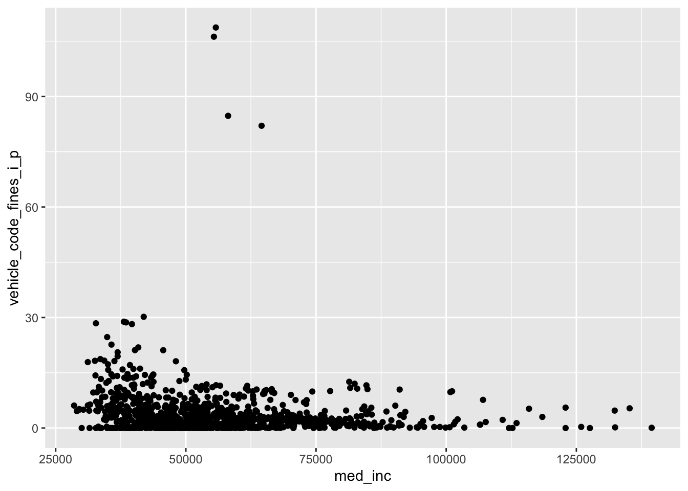

Correlation

Demo: What is the correlation between median household income and per capita traffic fines revenue?

# option 1
summarize(traffic_fines, r = cor(med_inc, vehicle_code_fines_i_p))

# A tibble: 1 × 1
       r
   <dbl>
1 -0.129

# option 2
cor(traffic_fines$med_inc, traffic_fines$vehicle_code_fines_i_p)

[1] -0.1291805

Define the model

This is the population model that explains the relationship between median household income and per capita traffic fines revenue.

\[ \text{traffic fines} = \beta_0 + \beta_1 \times \text{median household income} \]

Demo: Fit the linear regression model and display the results.

Tip

Use tidy() to print the model output in a readable, tabular format.

fines_inc_fit <- linear_reg() |>
  fit(vehicle_code_fines_i_p ~ med_inc, data = traffic_fines)

tidy(fines_inc_fit)

# A tibble: 2 × 5
  term          estimate std.error statistic  p.value
  <chr>            <dbl>     <dbl>     <dbl>    <dbl>
1 (Intercept)  6.93      0.762          9.10 4.45e-19
2 med_inc     -0.0000546 0.0000131     -4.17 3.35e- 5

# visualize the model
ggplot(
  data = traffic_fines,
  mapping = aes(x = med_inc, y = vehicle_code_fines_i_p)
) +
  geom_point() +
  geom_smooth(method = "lm")

`geom_smooth()` using formula = 'y ~ x'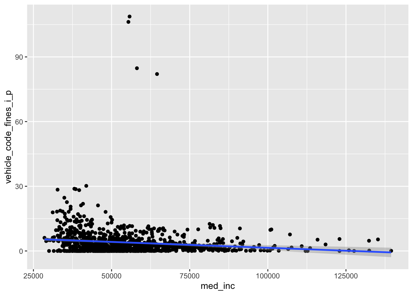

Your turn: Interpret the slope and the intercept in the context of the data.

Intercept: Add response here.
Slopes: Add response here.

Generate predictions

Your turn: What is the estimated per capita traffic fines revenue for a county with $80,000 median household income? What about a county with $15,000 median household income?

Tip

Use predict() to generate predicted values from a fitted model. Provide the new data in a data frame as the new_data argument.

Out-of-sample predictions

Be warned that even though we can generate predictions for any value of median household income, it is not always appropriate to do so. We should only generate predictions for values of the predictor variable that are within the range of the data used to fit the model (interpolation). $15,000 is outside of the range of the data (extrapolation).

predict(fines_inc_fit, new_data = tibble(med_inc = c(80000, 15000)))

# A tibble: 2 × 1
  .pred
  <dbl>
1  2.57
2  6.12

Conduct a hypothesis test

Your turn: State the hypotheses to evaluate the relationship between median household income and per capita traffic fines revenue.

Null hypothesis: Add response here.
Alternative hypothesis: Add response here.

Demo: Use permutation-based methods to conduct the hypothesis test.

# calculate observed fit
obs_fit <- traffic_fines |>
  specify(vehicle_code_fines_i_p ~ med_inc) |>
  fit()

# generate permuted null distribution
null_dist <- traffic_fines |>
  specify(vehicle_code_fines_i_p ~ med_inc) |>
  hypothesize(null = "independence") |>
  generate(reps = 1000, type = "permute") |>
  fit()

# visualize and calculate p-value
visualize(null_dist) +
  shade_p_value(obs_fit, direction = "both")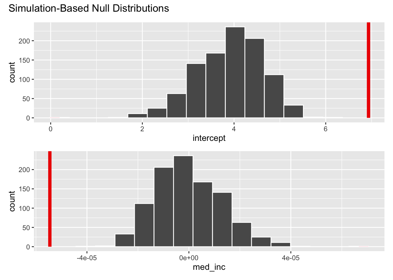

get_p_value(null_dist, obs_fit, direction = "both")

Warning: Please be cautious in reporting a p-value of 0. This result is an approximation
based on the number of `reps` chosen in the `generate()` step.
ℹ See `get_p_value()` (`?infer::get_p_value()`) for more information.
Please be cautious in reporting a p-value of 0. This result is an approximation
based on the number of `reps` chosen in the `generate()` step.
ℹ See `get_p_value()` (`?infer::get_p_value()`) for more information.

# A tibble: 2 × 2
  term      p_value
  <chr>       <dbl>
1 intercept       0
2 med_inc         0

Your turn: Interpret the $p$-value in context of the data and the research question. Use a significance level of 5%.

Add response here.

Estimate bootstrap confidence intervals for the slope

Demo: Estimate the 95% confidence interval for the slope of the relationship between median household income and per capita traffic fines revenue.

# bootstrap distribution for CIs
boot_full_dist <- traffic_fines |>
  specify(vehicle_code_fines_i_p ~ med_inc) |>
  generate(reps = 1000, type = "bootstrap") |>
  fit()

# get 95% confidence interval
conf_ints <- get_ci(boot_full_dist, level = 0.95, point_estimate = obs_fit)

visualize(boot_full_dist) +
  shade_confidence_interval(conf_ints)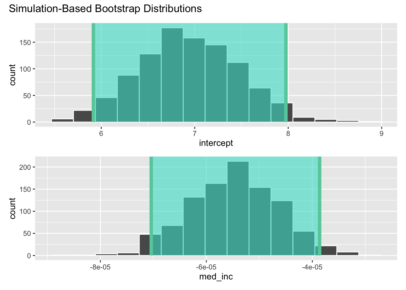

Your turn: How do we interpret this confidence interval?

Add response here.

Another model with a categorical explanatory variable

Your turn: Now let us ask the question we most care about: do politicians manipulate government policy during electoral years in an effort to gain an electoral advantage? In order to answer the question, we will examine the relationship between whether or not a sheriff election is held in the year and per capita traffic fines revenue.

Response variable: Add response here.
Predictor variable: Add response here.
Predictor type: Add response here.

Demo: Make an appropriate visualization to investigate this relationship below. Additionally, calculate the mean per capita traffic fines revenue for years that are and are not election years.

ggplot(
  data = traffic_fines,
  mapping = aes(x = elec_dummy, y = vehicle_code_fines_i_p)
) +
  geom_boxplot()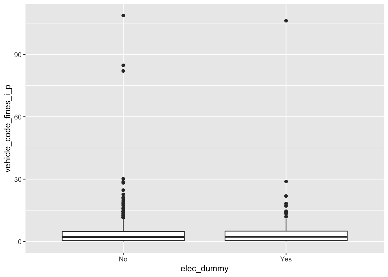

traffic_fines |>
  group_by(elec_dummy) |>
  summarize(mean_fines = mean(vehicle_code_fines_i_p, na.rm = TRUE))

# A tibble: 2 × 2
  elec_dummy mean_fines
  <chr>           <dbl>
1 No               3.90
2 Yes              3.91

Demo: Change the geom of your previous plot to geom_point(). Use this plot to think about how R models these data.

ggplot(
  data = traffic_fines,
  mapping = aes(x = elec_dummy, y = vehicle_code_fines_i_p)
) +
  geom_point()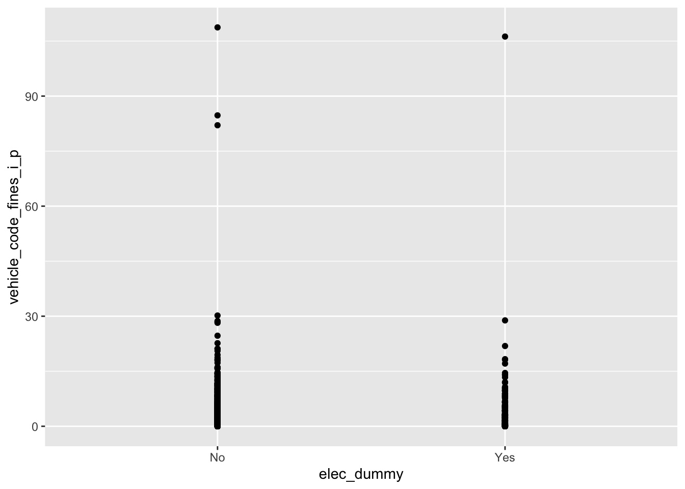

Your turn: Fit the linear regression model and display the results. Print the estimated model output below.

fines_elec_dummy_fit <- linear_reg() |>
  fit(vehicle_code_fines_i_p ~ elec_dummy, data = traffic_fines)

tidy(fines_elec_dummy_fit)

# A tibble: 2 × 5
  term          estimate std.error statistic  p.value
  <chr>            <dbl>     <dbl>     <dbl>    <dbl>
1 (Intercept)     3.90       0.256   15.2    2.84e-47
2 elec_dummyYes   0.0171     0.543    0.0315 9.75e- 1

Demo: Interpret the slope and the intercept in the context of the data.

Intercept: Add response here.
Slope: Add response here.

Conduct a hypothesis test

Your turn: State the hypotheses to evaluate the relationship between median household income and per capita traffic fines revenue.

Null hypothesis: Add response here.
Alternative hypothesis: Add response here.

\[H_A: \beta_1 \neq 0\]

Demo: Use permutation-based methods to conduct the hypothesis test.

# calculate observed fit
obs_fit <- traffic_fines |>
  specify(vehicle_code_fines_i_p ~ elec_dummy) |>
  fit()

# generate permuted null distribution
null_dist <- traffic_fines |>
  specify(vehicle_code_fines_i_p ~ elec_dummy) |>
  hypothesize(null = "independence") |>
  generate(reps = 1000, type = "permute") |>
  fit()

# visualize and calculate p-value
visualize(null_dist) +
  shade_p_value(obs_fit, direction = "both")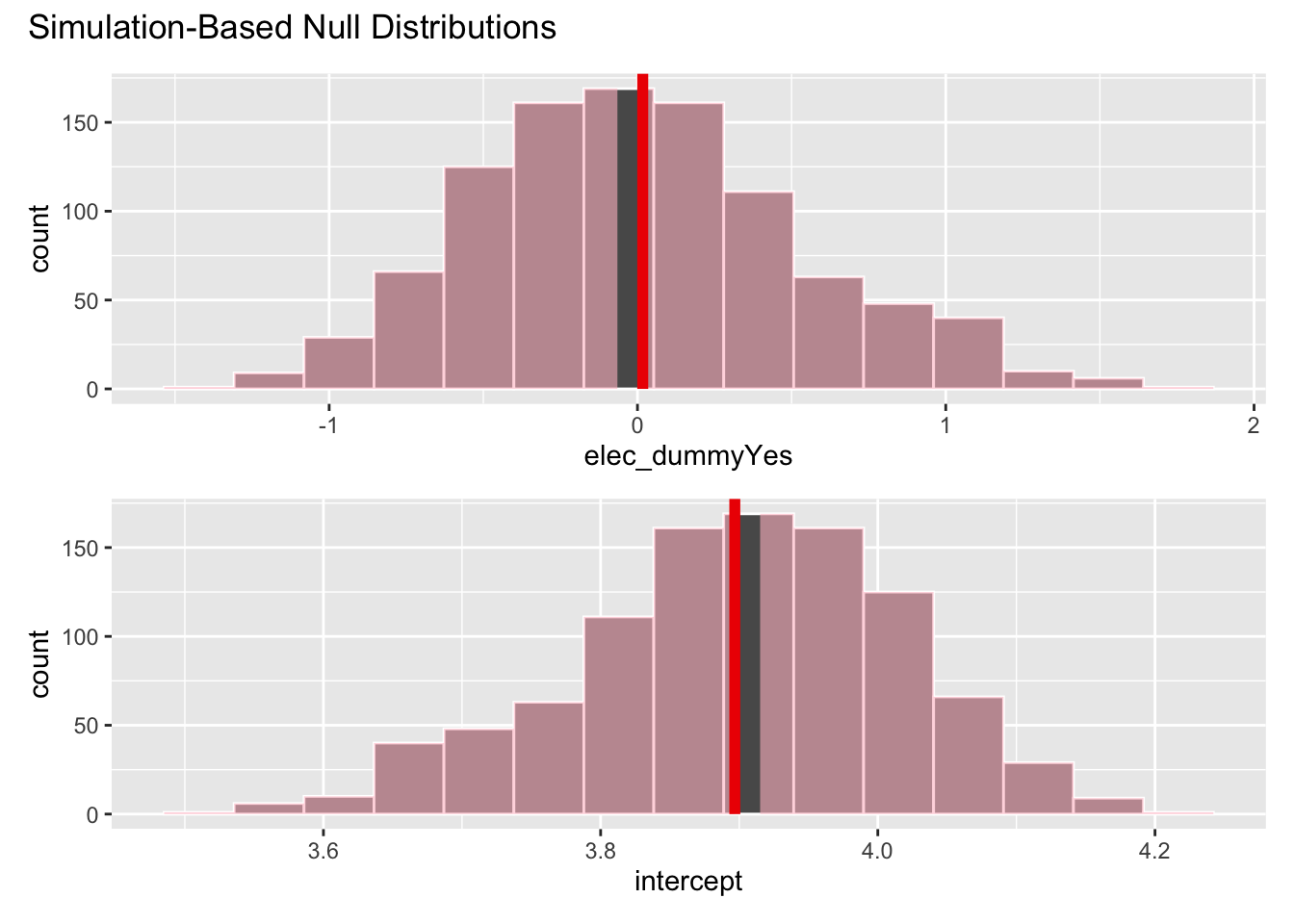

get_p_value(null_dist, obs_fit, direction = "both")

# A tibble: 2 × 2
  term          p_value
  <chr>           <dbl>
1 elec_dummyYes   0.942
2 intercept       0.942

Your turn: Interpret the $p$-value in context of the data and the research question. Use a significance level of 5%.

Add response here.

Check model conditions

Recall the technical conditions for linear regression:

L: linear model
I: independent observations
N: points are normally distributed around the line
E: equal variability around the line for all values of the explanatory variable

Your turn: Check the linearity assumption for the model with elec_dummy as the predictor. Examine the residuals to assist you with this process.

# augment() allows us to extract observation-level statistics from a model object
fines_elec_dummy_aug <- augment(fines_elec_dummy_fit, new_data = traffic_fines)
fines_elec_dummy_aug

# A tibble: 1,025 × 8
   .pred .resid  year county_code county_name vehicle_code_fines_i_p med_inc
   <dbl>  <dbl> <dbl>       <dbl> <chr>                        <dbl>   <dbl>
 1  3.90 -0.507  2003           1 Alameda                       3.39   56225
 2  3.90 -0.107  2004           1 Alameda                       3.79   57659
 3  3.90 -0.899  2005           1 Alameda                       3.00   60937
 4  3.91 -0.639  2006           1 Alameda                       3.27   64285
 5  3.90 -0.591  2007           1 Alameda                       3.31   68263
 6  3.90 -0.388  2008           1 Alameda                       3.51   70217
 7  3.90 -0.276  2009           1 Alameda                       3.62   68258
 8  3.91 -0.713  2010           1 Alameda                       3.20   66937
 9  3.90 -1.15   2011           1 Alameda                       2.75   67295
10  3.90 -1.63   2012           1 Alameda                       2.27   70209
# ℹ 1,015 more rows
# ℹ 1 more variable: elec_dummy <chr>

# the linear regression model
ggplot(
  data = fines_elec_dummy_aug,
  mapping = aes(
    x = as.numeric(elec_dummy == "Yes"),
    y = vehicle_code_fines_i_p
  )
) +
  geom_point() +
  geom_smooth(method = "lm")

`geom_smooth()` using formula = 'y ~ x'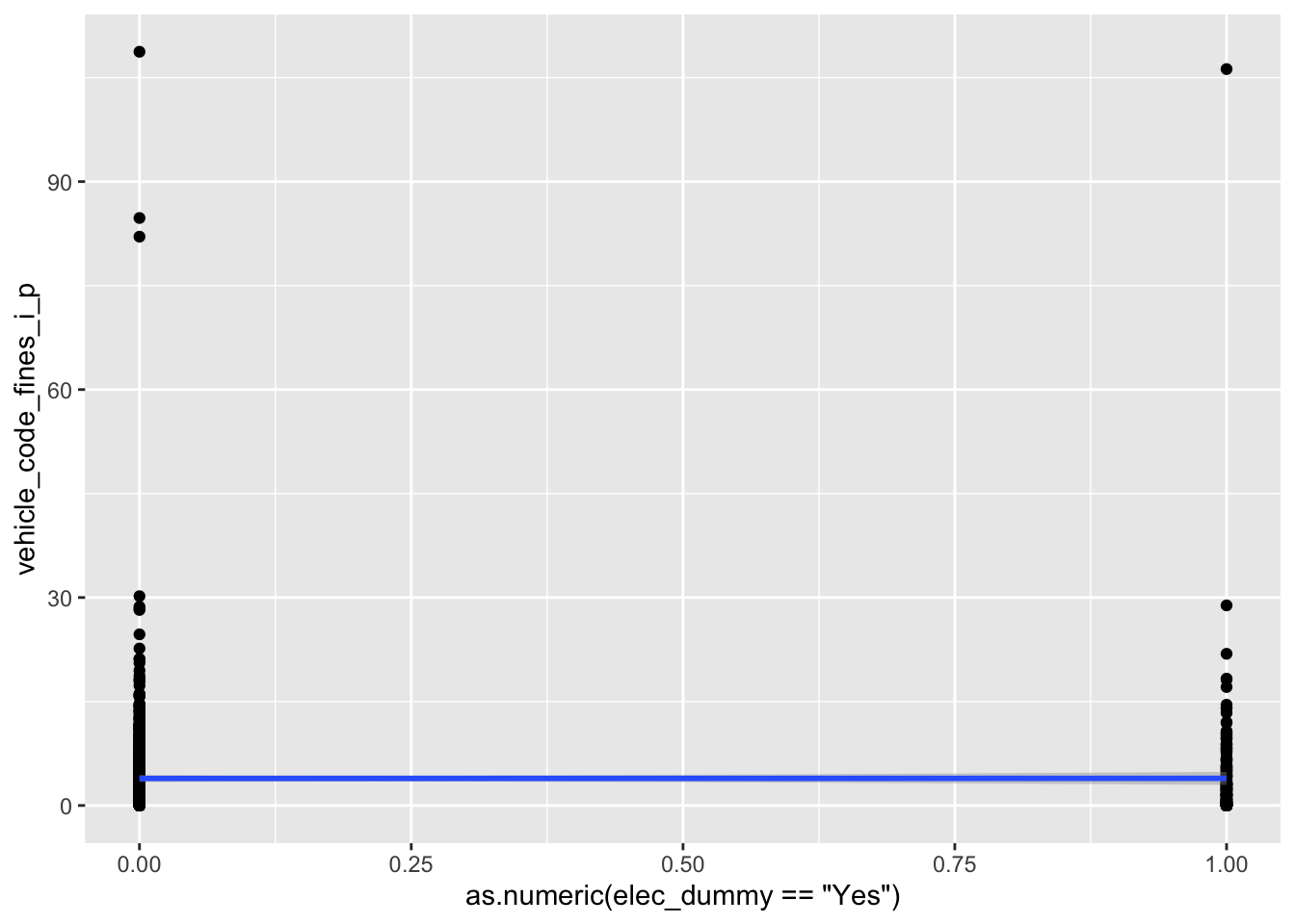

# distribution of the residuals
ggplot(data = fines_elec_dummy_aug, mapping = aes(x = .resid)) +
  geom_histogram()

`stat_bin()` using `bins = 30`. Pick better value `binwidth`.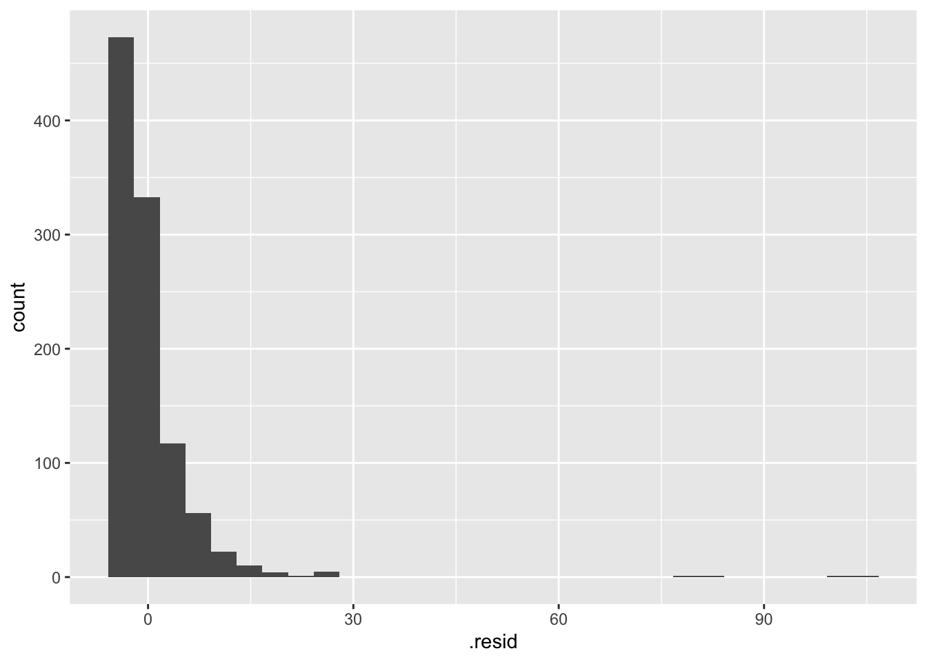

# use the .resid column to plot the predicted values vs. the residuals
# jitter because the explanatory variable only has 2 unique values
ggplot(data = fines_elec_dummy_aug, mapping = aes(x = .pred, y = .resid)) +
  geom_jitter() +
  geom_hline(yintercept = 0, linetype = "dashed")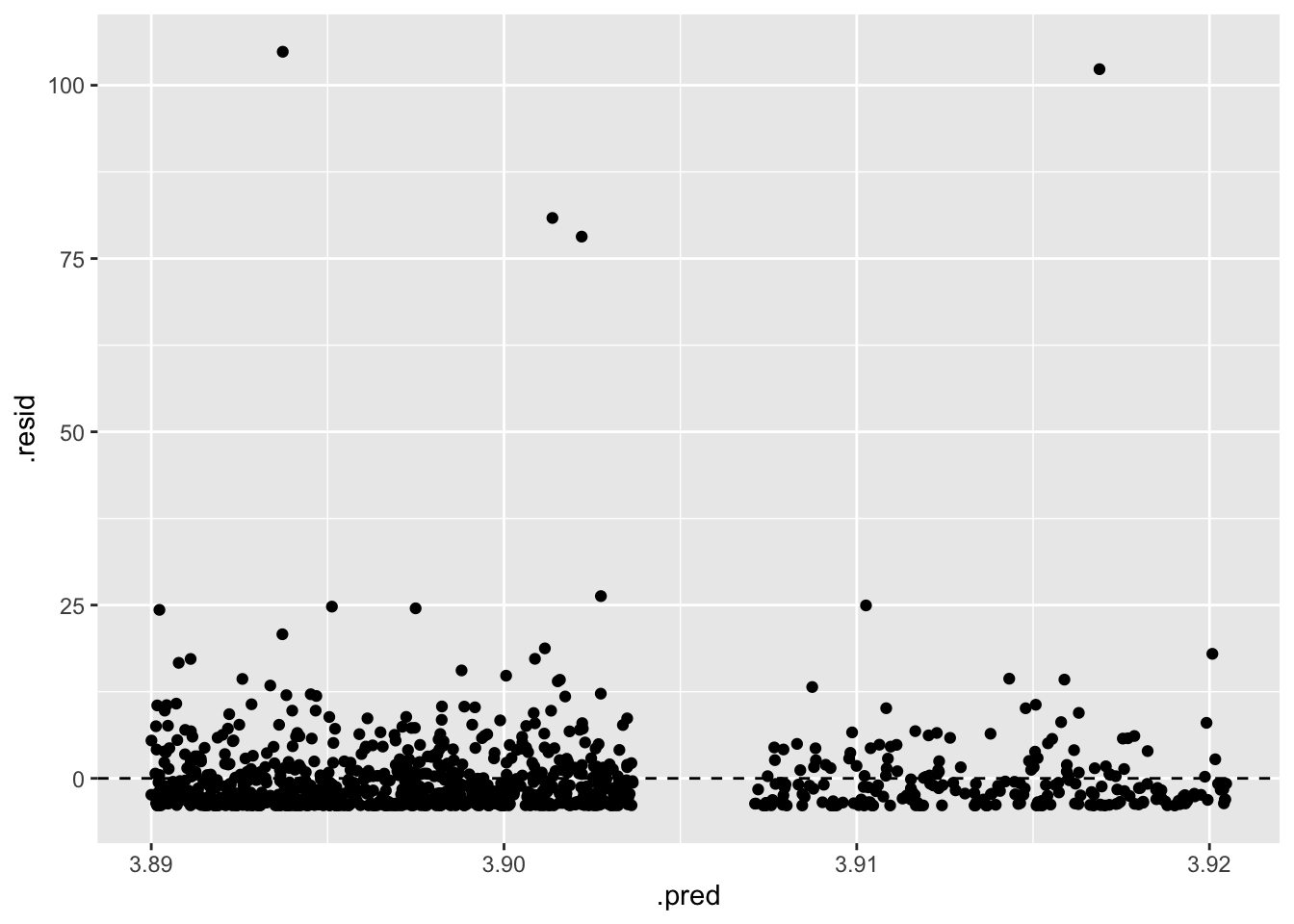

L: linear model - Add response here.
I: independent observations - Add response here.
N: points are normally distributed around the line - Add response here.
E: equal variability around the line for all values of the explanatory variable - Add response here.

Footnotes

Su, Min, and Christian Buerger. 2025. “Playing politics with traffic fines: Sheriff elections and political cycles in traffic fines revenue.” American Journal of Political Science 69: 164–175. https://doi.org/10.1111/ajps.12866↩︎
The codebook is available from Dataverse. The data set has been lightly cleaned for the application exercise.↩︎