AE 08: Using {duckdb} for NYC flights
Suggested answers
Packages
We will use the following packages in this application exercise.
- {tidyverse}: For data import, wrangling, and visualization.
- {duckdb}: To query a DuckDB.
- {dbplyr}: To translate our {dplyr} and {tidyr} functions to SQL.
- {scales}: Formatting graph labels.
New York City flights data
The U.S. Department of Transportation publishes detailed statistics on flights originating in the United States. {nycflights13} is a highly popular R package containing information on all flights that departed NYC1 in 2013. The package was originally developed to provide practice wrangling and working with relational datasets.
1 Specifically, John F. Kennedy International Airport (JFK), LaGuardia Airport (LGA), and Newark International Airport (EWR).
That said, this package has become quite dated since it was originally developed in the mid-2010s. The same air travel data can be accessed for any airports in the United States using the {anyflights} package. The challenge is that data for more than a trivial handful of airports and years becomes significantly large and unwieldy to utilize.
To solve these issues, we will utilize a DuckDB that contains detailed air travel data for all NYC airports from 2015-2023. This dataset can be access from data/nyc-flights.duckdb.
Connect to the database
Demonstration: Connect to the local database and identify the tables.
con <- duckdb(dbdir = "data/nyc-flights.duckdb") |>
dbConnect()
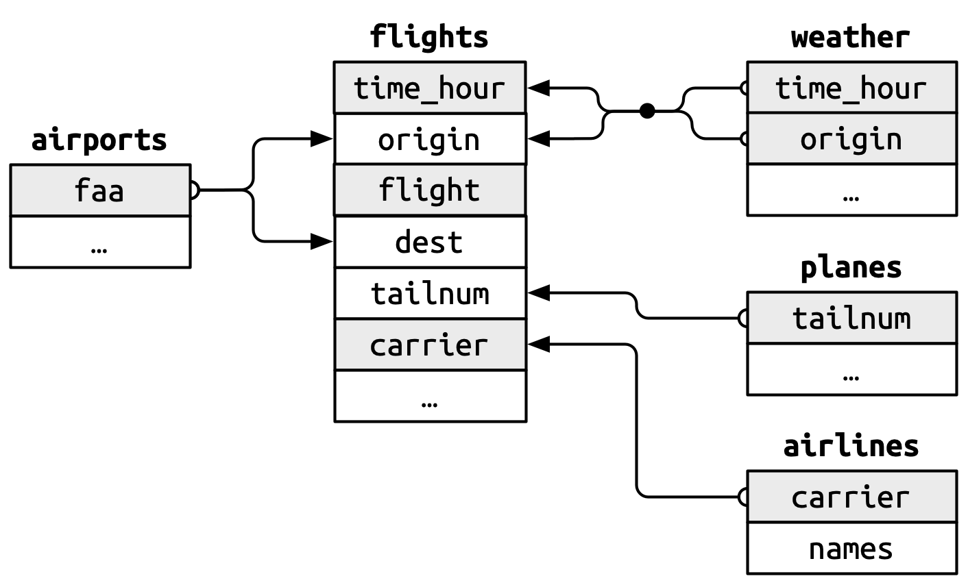
dbListTables(con)[1] "airlines" "airports" "flights" "planes" "weather" The database has the following relational structure:
Demonstration: Use tbl() to create an object that represents each database table. This will allow us to use {dbplyr} to translate our code to the corresponding SQL query.
Translate some basic SQL queries
Your turn: Explain what each of the following SQL queries does, and recreate them using {dbplyr}.
SELECT flights.*
FROM flights
WHERE (dep_delay < arr_delay)
Add response here. Filter the flights table to only keep rows where the departure delay is smaller than the arrival delay.
flights |>
  filter(dep_delay < arr_delay) |>
  show_query()
<SQL>
SELECT flights.*
FROM flights
WHERE (dep_delay < arr_delay)SELECT flights.*, distance / (air_time / 60.0) AS speed
FROM flightsAdd response here. Create a new variable in the flights table called speed which is the distance traveled divided by the air time (in hours).
flights |>
mutate(speed = distance / (air_time / 60)) |>
show_query()<SQL>
SELECT flights.*, distance / (air_time / 60.0) AS speed
FROM flightsWhat causes flight delays?
Your turn: What is the relationship between weather events and departure delays? Calculate the average departure delay and join with the weather table. How do these R commands translate to SQL? What trends do you see?
- Before summarizing
flights, examine theweathertable and figure out its unit of analysis. This will clue you in to how best to summarize theflightsdata. - Use
show_query()to examine the translated SQL code.
# examine one weather event - wind speed
wind_delay <- flights |>
  group_by(origin, year, month, day, hour) |>
  summarize(dep_delay = mean(dep_delay)) |>
  left_join(y = weather)

# what was the SQL query?
show_query(wind_delay)
<SQL>
SELECT
LHS.*,
"temp",
dewp,
humid,
wind_dir,
wind_speed,
wind_gust,
precip,
pressure,
visib,
time_hour
FROM (
SELECT origin, "year", "month", "day", "hour", AVG(dep_delay) AS dep_delay
FROM flights
GROUP BY origin, "year", "month", "day", "hour"
) LHS
LEFT JOIN weather
ON (
LHS.origin = weather.origin AND
LHS."year" = weather."year" AND
LHS."month" = weather."month" AND
LHS."day" = weather."day" AND
LHS."hour" = weather."hour"
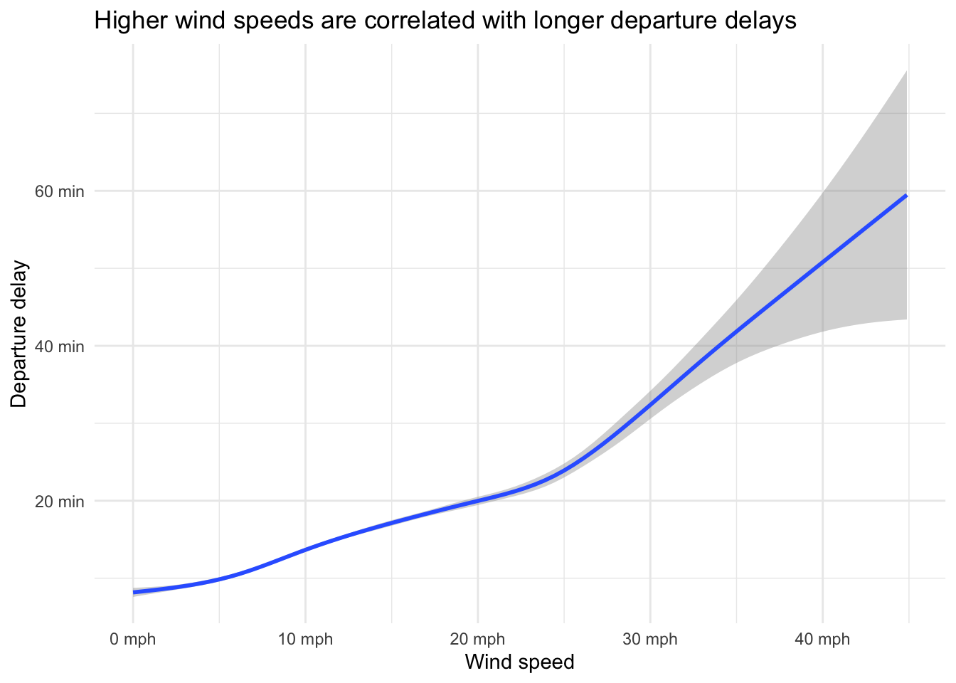
)# visualize as a plot
ggplot(data = wind_delay, mapping = aes(x = wind_speed, y = dep_delay)) +
geom_smooth() +
scale_x_continuous(labels = label_number(scale_cut = cut_si(unit = "mph"))) +
scale_y_continuous(labels = label_number(scale_cut = cut_si(unit = "min"))) +
labs(
title = "Higher wind speeds are correlated with longer departure delays",
x = "Wind speed",
y = "Departure delay"
)
# look at all simultaneously
weather_delay <- wind_delay |>
  pivot_longer(
    cols = temp:visib,
    names_to = "variable",
    values_to = "value"
  )

# what was the SQL query?
show_query(weather_delay)
<SQL>
SELECT
origin,
"year",
"month",
"day",
"hour",
dep_delay,
time_hour,
'temp' AS "variable",
"temp" AS "value"
FROM (
SELECT
LHS.*,
"temp",
dewp,
humid,
wind_dir,
wind_speed,
wind_gust,
precip,
pressure,
visib,
time_hour
FROM (
SELECT origin, "year", "month", "day", "hour", AVG(dep_delay) AS dep_delay
FROM flights
GROUP BY origin, "year", "month", "day", "hour"
) LHS
LEFT JOIN weather
ON (
LHS.origin = weather.origin AND
LHS."year" = weather."year" AND
LHS."month" = weather."month" AND
LHS."day" = weather."day" AND
LHS."hour" = weather."hour"
)
) q01
UNION ALL
SELECT
origin,
"year",
"month",
"day",
"hour",
dep_delay,
time_hour,
'dewp' AS "variable",
dewp AS "value"
FROM (
SELECT
LHS.*,
"temp",
dewp,
humid,
wind_dir,
wind_speed,
wind_gust,
precip,
pressure,
visib,
time_hour
FROM (
SELECT origin, "year", "month", "day", "hour", AVG(dep_delay) AS dep_delay
FROM flights
GROUP BY origin, "year", "month", "day", "hour"
) LHS
LEFT JOIN weather
ON (
LHS.origin = weather.origin AND
LHS."year" = weather."year" AND
LHS."month" = weather."month" AND
LHS."day" = weather."day" AND
LHS."hour" = weather."hour"
)
) q01
UNION ALL
SELECT
origin,
"year",
"month",
"day",
"hour",
dep_delay,
time_hour,
'humid' AS "variable",
humid AS "value"
FROM (
SELECT
LHS.*,
"temp",
dewp,
humid,
wind_dir,
wind_speed,
wind_gust,
precip,
pressure,
visib,
time_hour
FROM (
SELECT origin, "year", "month", "day", "hour", AVG(dep_delay) AS dep_delay
FROM flights
GROUP BY origin, "year", "month", "day", "hour"
) LHS
LEFT JOIN weather
ON (
LHS.origin = weather.origin AND
LHS."year" = weather."year" AND
LHS."month" = weather."month" AND
LHS."day" = weather."day" AND
LHS."hour" = weather."hour"
)
) q01
UNION ALL
SELECT
origin,
"year",
"month",
"day",
"hour",
dep_delay,
time_hour,
'wind_dir' AS "variable",
wind_dir AS "value"
FROM (
SELECT
LHS.*,
"temp",
dewp,
humid,
wind_dir,
wind_speed,
wind_gust,
precip,
pressure,
visib,
time_hour
FROM (
SELECT origin, "year", "month", "day", "hour", AVG(dep_delay) AS dep_delay
FROM flights
GROUP BY origin, "year", "month", "day", "hour"
) LHS
LEFT JOIN weather
ON (
LHS.origin = weather.origin AND
LHS."year" = weather."year" AND
LHS."month" = weather."month" AND
LHS."day" = weather."day" AND
LHS."hour" = weather."hour"
)
) q01
UNION ALL
SELECT
origin,
"year",
"month",
"day",
"hour",
dep_delay,
time_hour,
'wind_speed' AS "variable",
wind_speed AS "value"
FROM (
SELECT
LHS.*,
"temp",
dewp,
humid,
wind_dir,
wind_speed,
wind_gust,
precip,
pressure,
visib,
time_hour
FROM (
SELECT origin, "year", "month", "day", "hour", AVG(dep_delay) AS dep_delay
FROM flights
GROUP BY origin, "year", "month", "day", "hour"
) LHS
LEFT JOIN weather
ON (
LHS.origin = weather.origin AND
LHS."year" = weather."year" AND
LHS."month" = weather."month" AND
LHS."day" = weather."day" AND
LHS."hour" = weather."hour"
)
) q01
UNION ALL
SELECT
origin,
"year",
"month",
"day",
"hour",
dep_delay,
time_hour,
'wind_gust' AS "variable",
wind_gust AS "value"
FROM (
SELECT
LHS.*,
"temp",
dewp,
humid,
wind_dir,
wind_speed,
wind_gust,
precip,
pressure,
visib,
time_hour
FROM (
SELECT origin, "year", "month", "day", "hour", AVG(dep_delay) AS dep_delay
FROM flights
GROUP BY origin, "year", "month", "day", "hour"
) LHS
LEFT JOIN weather
ON (
LHS.origin = weather.origin AND
LHS."year" = weather."year" AND
LHS."month" = weather."month" AND
LHS."day" = weather."day" AND
LHS."hour" = weather."hour"
)
) q01
UNION ALL
SELECT
origin,
"year",
"month",
"day",
"hour",
dep_delay,
time_hour,
'precip' AS "variable",
precip AS "value"
FROM (
SELECT
LHS.*,
"temp",
dewp,
humid,
wind_dir,
wind_speed,
wind_gust,
precip,
pressure,
visib,
time_hour
FROM (
SELECT origin, "year", "month", "day", "hour", AVG(dep_delay) AS dep_delay
FROM flights
GROUP BY origin, "year", "month", "day", "hour"
) LHS
LEFT JOIN weather
ON (
LHS.origin = weather.origin AND
LHS."year" = weather."year" AND
LHS."month" = weather."month" AND
LHS."day" = weather."day" AND
LHS."hour" = weather."hour"
)
) q01
UNION ALL
SELECT
origin,
"year",
"month",
"day",
"hour",
dep_delay,
time_hour,
'pressure' AS "variable",
pressure AS "value"
FROM (
SELECT
LHS.*,
"temp",
dewp,
humid,
wind_dir,
wind_speed,
wind_gust,
precip,
pressure,
visib,
time_hour
FROM (
SELECT origin, "year", "month", "day", "hour", AVG(dep_delay) AS dep_delay
FROM flights
GROUP BY origin, "year", "month", "day", "hour"
) LHS
LEFT JOIN weather
ON (
LHS.origin = weather.origin AND
LHS."year" = weather."year" AND
LHS."month" = weather."month" AND
LHS."day" = weather."day" AND
LHS."hour" = weather."hour"
)
) q01
UNION ALL
SELECT
origin,
"year",
"month",
"day",
"hour",
dep_delay,
time_hour,
'visib' AS "variable",
visib AS "value"
FROM (
SELECT
LHS.*,
"temp",
dewp,
humid,
wind_dir,
wind_speed,
wind_gust,
precip,
pressure,
visib,
time_hour
FROM (
SELECT origin, "year", "month", "day", "hour", AVG(dep_delay) AS dep_delay
FROM flights
GROUP BY origin, "year", "month", "day", "hour"
) LHS
LEFT JOIN weather
ON (
LHS.origin = weather.origin AND
LHS."year" = weather."year" AND
LHS."month" = weather."month" AND
LHS."day" = weather."day" AND
LHS."hour" = weather."hour"
)
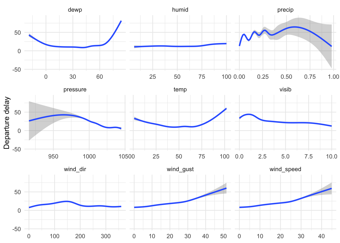
) q01# visualize as a plot
ggplot(data = weather_delay, mapping = aes(x = value, y = dep_delay)) +
geom_smooth() +
facet_wrap(facets = vars(variable), scales = "free_x") +
labs(
x = NULL,
y = "Departure delay"
)
Number of flights departing NYC airports over time
Now let’s examine potential patterns or trends in the volume of flights departing NYC-area airports over time.
Create a date variable
Your turn: Currently flights does not have a standalone date variable that identifies the date of the flight. Create one and store it at the beginning of the table.
lubridate::make_date() can create a date variable from numeric columns which contain each of the date components.
flights <- flights |>
  mutate(date = make_date(year = year, month = month, day = day), .before = everything())
show_query(flights)
<SQL>
SELECT make_date("year", "month", "day") AS date, flights.*
FROM flightsVisualize the volume of flights over time
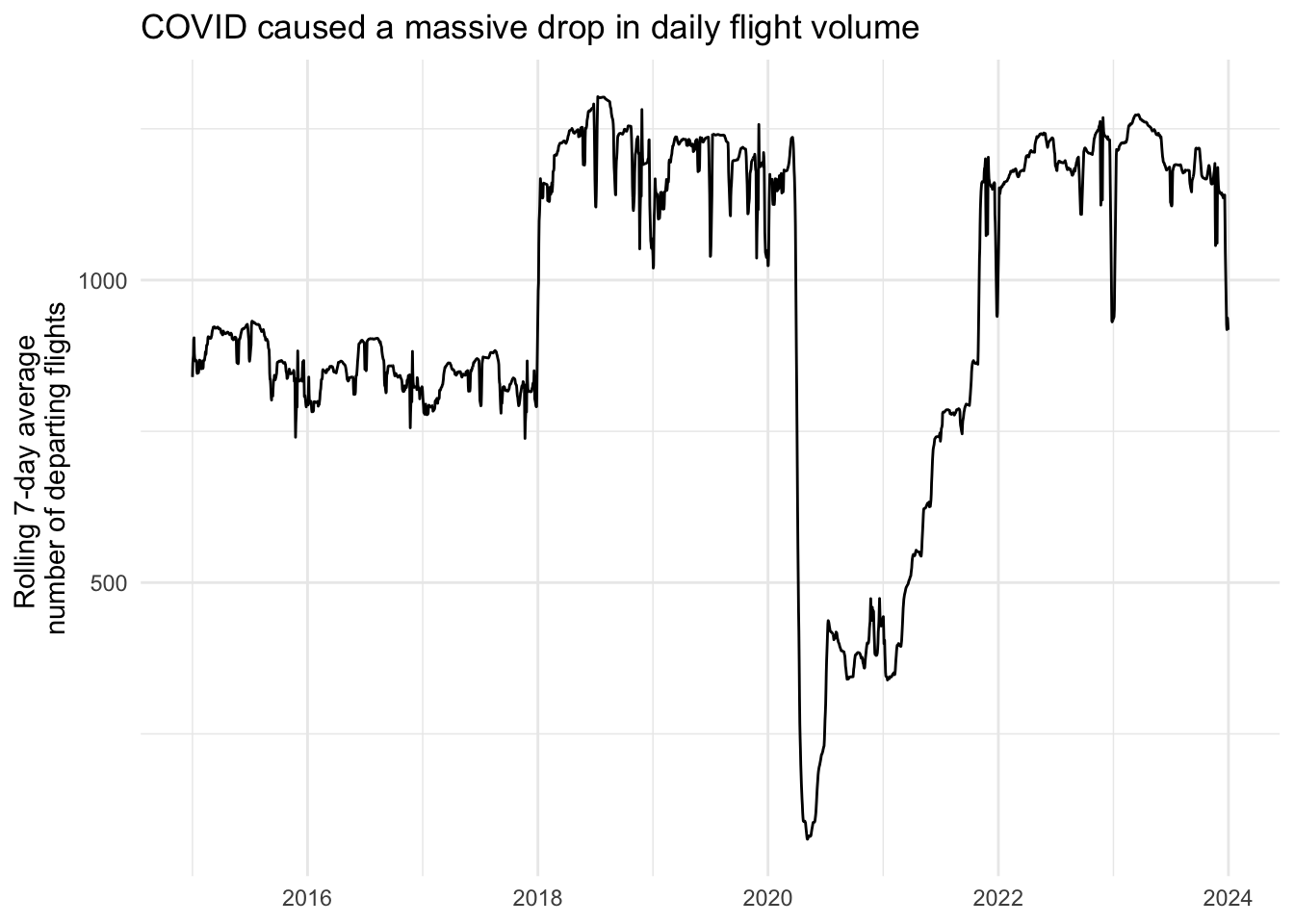
Demonstration: Calculate the daily number of departing flights from NYC and visualize as a line graph.
flights |>
  count(date) |>
  ggplot(mapping = aes(x = date, y = n)) +
  geom_line() +
  labs(
    title = "COVID caused a massive drop in daily flight volume",
    x = NULL,
    y = "Number of departing flights"
  )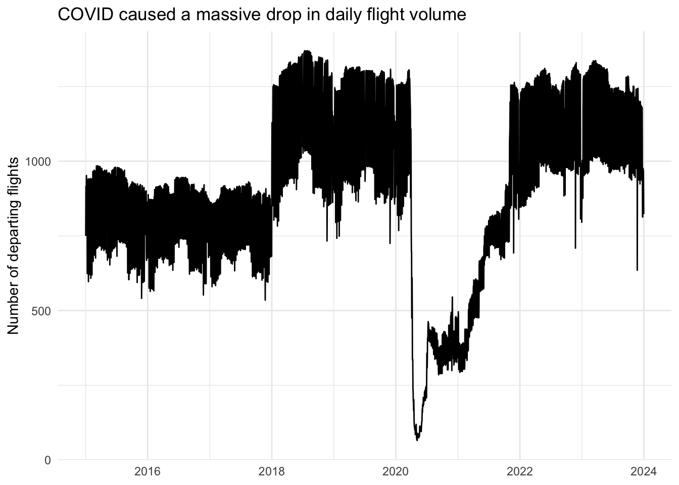
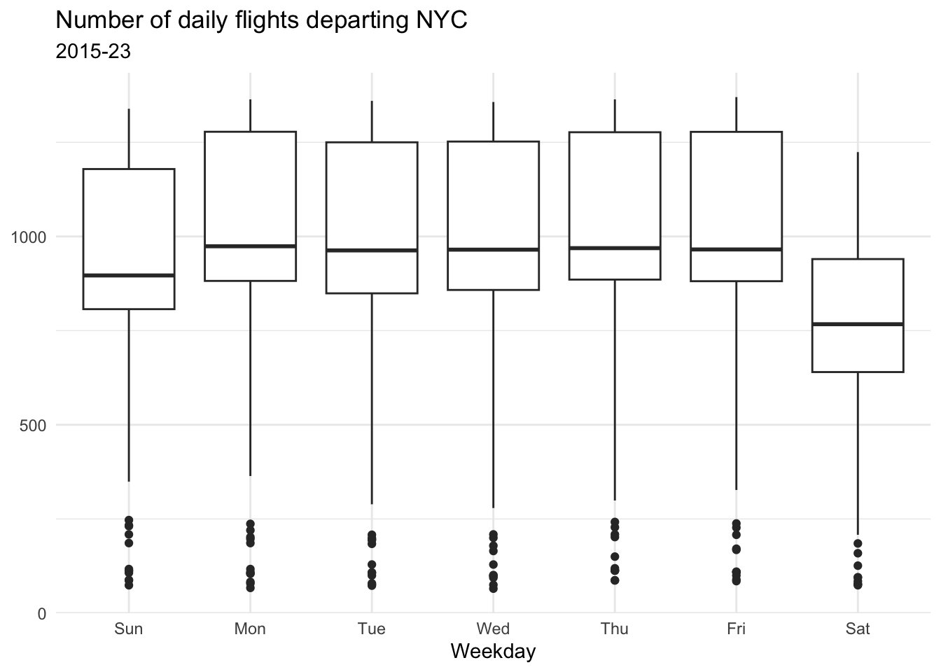
This line graph is very noisy due to cyclical fluctuations in flight frequency.2 One method to smooth this out is to create a rolling average. This generates a sliding window across the timespan, averaging the values for each observation within that span as it moves across the time period.
Primarily, the number of daily flights drops substantially on Sundays.
There are several ways to accomplish this task in R. One popular implementation in the {zoo} package provides drop in functions for calculating rolling means, maximums, medians, and sums. Unfortunately these functions have not been translated by {dbplyr} for use with SQL databases.
Fortunately SQL has direct support for these operations through so-called window functions. In order to utilize them, we need to identify the boundaries of the frame (the sliding window). We can do that using window_frame().
Demonstration: Calculate a rolling seven-day average number of flights departing from NYC.
roll_flights <- flights |>
  count(date) |>
  window_frame(-3, 3) |>
  mutate(roll_n = mean(n))

show_query(roll_flights)
Warning: Named arguments ignored for SQL make_dateWarning: Windowed expression `AVG(n)` does not have explicit order.
ℹ Please use `arrange()` or `window_order()` to make deterministic.<SQL>
SELECT q01.*, AVG(n) OVER (ROWS BETWEEN 3 PRECEDING AND 3 FOLLOWING) AS roll_n
FROM (
SELECT date, COUNT(*) AS n
FROM (
SELECT make_date("year", "month", "day") AS date, flights.*
FROM flights
) q01
GROUP BY date
) q01collect(roll_flights)Warning: Named arguments ignored for SQL make_date
Windowed expression `AVG(n)` does not have explicit order.
ℹ Please use `arrange()` or `window_order()` to make deterministic.# A tibble: 3,287 × 3
date n roll_n
<date> <dbl> <dbl>
1 2015-01-02 916 863.
2 2015-01-03 804 870.
3 2015-01-11 835 874
4 2015-01-13 898 844.
5 2015-01-27 895 852.
6 2015-01-28 896 873.
7 2015-02-14 665 888.
8 2015-02-20 970 898.
9 2015-02-24 949 909.
10 2015-02-25 942 907.
# ℹ 3,277 more rowsWarning: Named arguments ignored for SQL make_date
Windowed expression `AVG(n)` does not have explicit order.
ℹ Please use `arrange()` or `window_order()` to make deterministic.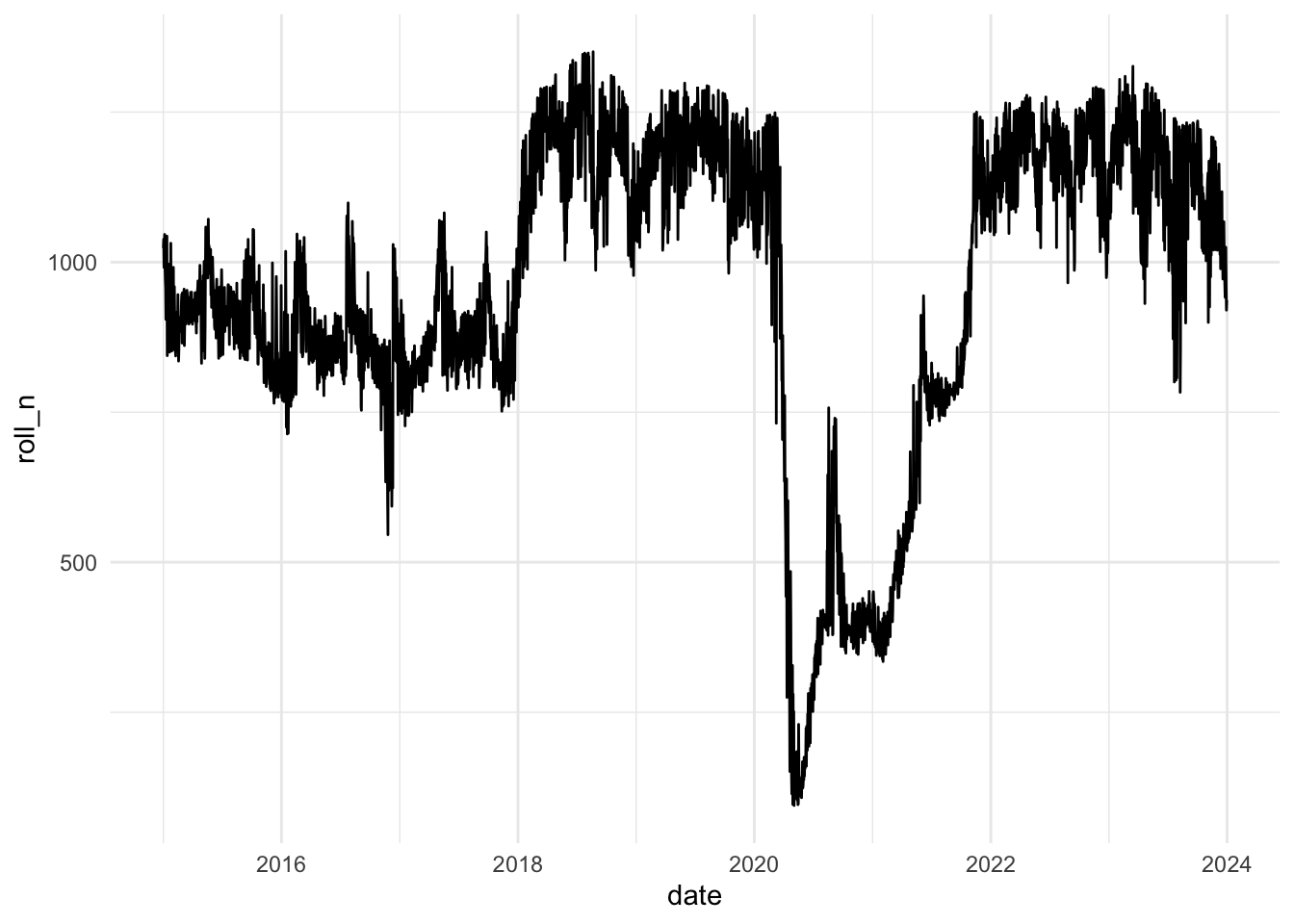
Unfortunately this is only partially correct. Recall that SQL tables have no intrinsic row-order. Every time you run a query, the rows you obtain can be in a different order every time. In order to ensure we correctly calculate the seven-day window, we need to define the order of the rows for the table. We can do this by either using arrange() to explicitly order the rows before using the window function, or use window_order() to define the order.
roll_flights <- flights |>
  count(date) |>
  window_order(date) |>
  window_frame(-3, 3) |>
  mutate(roll_n = mean(n))

show_query(roll_flights)
<SQL>
SELECT
q01.*,
AVG(n) OVER (ORDER BY date ROWS BETWEEN 3 PRECEDING AND 3 FOLLOWING) AS roll_n
FROM (
SELECT date, COUNT(*) AS n
FROM (
SELECT make_date("year", "month", "day") AS date, flights.*
FROM flights
) q01
GROUP BY date
) q01ggplot(data = roll_flights, mapping = aes(x = date, y = roll_n)) +
geom_line() +
labs(
title = "COVID caused a massive drop in daily flight volume",
x = NULL,
y = "Rolling 7-day average \nnumber of departing flights"
)
sessioninfo::session_info()─ Session info ───────────────────────────────────────────────────────────────
setting value
version R version 4.4.2 (2024-10-31)
os macOS Sonoma 14.6.1
system aarch64, darwin20
ui X11
language (EN)
collate en_US.UTF-8
ctype en_US.UTF-8
tz America/New_York
date 2025-02-26
pandoc 3.4 @ /usr/local/bin/ (via rmarkdown)
─ Packages ───────────────────────────────────────────────────────────────────
package * version date (UTC) lib source
blob 1.2.4 2023-03-17 [1] CRAN (R 4.3.0)
cli 3.6.3 2024-06-21 [1] CRAN (R 4.4.0)
DBI * 1.2.3 2024-06-02 [1] CRAN (R 4.4.0)
dbplyr * 2.5.0 2024-03-19 [1] CRAN (R 4.3.1)
dichromat 2.0-0.1 2022-05-02 [1] CRAN (R 4.3.0)
digest 0.6.37 2024-08-19 [1] CRAN (R 4.4.1)
dplyr * 1.1.4 2023-11-17 [1] CRAN (R 4.3.1)
duckdb * 1.1.3-2 2025-01-24 [1] CRAN (R 4.4.1)
evaluate 1.0.3 2025-01-10 [1] CRAN (R 4.4.1)
farver 2.1.2 2024-05-13 [1] CRAN (R 4.3.3)
fastmap 1.2.0 2024-05-15 [1] CRAN (R 4.4.0)
forcats * 1.0.0 2023-01-29 [1] CRAN (R 4.3.0)
generics 0.1.3 2022-07-05 [1] CRAN (R 4.3.0)
ggplot2 * 3.5.1 2024-04-23 [1] CRAN (R 4.3.1)
glue 1.8.0 2024-09-30 [1] CRAN (R 4.4.1)
gtable 0.3.6 2024-10-25 [1] CRAN (R 4.4.1)
here 1.0.1 2020-12-13 [1] CRAN (R 4.3.0)
hms 1.1.3 2023-03-21 [1] CRAN (R 4.3.0)
htmltools 0.5.8.1 2024-04-04 [1] CRAN (R 4.3.1)
htmlwidgets 1.6.4 2023-12-06 [1] CRAN (R 4.3.1)
jsonlite 1.8.9 2024-09-20 [1] CRAN (R 4.4.1)
knitr 1.49 2024-11-08 [1] CRAN (R 4.4.1)
labeling 0.4.3 2023-08-29 [1] CRAN (R 4.3.0)
lattice 0.22-6 2024-03-20 [1] CRAN (R 4.4.2)
lifecycle 1.0.4 2023-11-07 [1] CRAN (R 4.3.1)
lubridate * 1.9.3 2023-09-27 [1] CRAN (R 4.3.1)
magrittr 2.0.3 2022-03-30 [1] CRAN (R 4.3.0)
Matrix 1.7-1 2024-10-18 [1] CRAN (R 4.4.2)
mgcv 1.9-1 2023-12-21 [1] CRAN (R 4.4.2)
nlme 3.1-166 2024-08-14 [1] CRAN (R 4.4.2)
pillar 1.10.1 2025-01-07 [1] CRAN (R 4.4.1)
pkgconfig 2.0.3 2019-09-22 [1] CRAN (R 4.3.0)
purrr * 1.0.2 2023-08-10 [1] CRAN (R 4.3.0)
R6 2.5.1 2021-08-19 [1] CRAN (R 4.3.0)
RColorBrewer 1.1-3 2022-04-03 [1] CRAN (R 4.3.0)
readr * 2.1.5 2024-01-10 [1] CRAN (R 4.3.1)
rlang 1.1.5 2025-01-17 [1] CRAN (R 4.4.1)
rmarkdown 2.29 2024-11-04 [1] CRAN (R 4.4.1)
rprojroot 2.0.4 2023-11-05 [1] CRAN (R 4.3.1)
scales * 1.3.0.9000 2024-11-14 [1] Github (r-lib/scales@ee03582)
sessioninfo 1.2.2 2021-12-06 [1] CRAN (R 4.3.0)
stringi 1.8.4 2024-05-06 [1] CRAN (R 4.3.1)
stringr * 1.5.1 2023-11-14 [1] CRAN (R 4.3.1)
tibble * 3.2.1 2023-03-20 [1] CRAN (R 4.3.0)
tidyr * 1.3.1 2024-01-24 [1] CRAN (R 4.3.1)
tidyselect 1.2.1 2024-03-11 [1] CRAN (R 4.3.1)
tidyverse * 2.0.0 2023-02-22 [1] CRAN (R 4.3.0)
timechange 0.3.0 2024-01-18 [1] CRAN (R 4.3.1)
tzdb 0.4.0 2023-05-12 [1] CRAN (R 4.3.0)
vctrs 0.6.5 2023-12-01 [1] CRAN (R 4.3.1)
withr 3.0.2 2024-10-28 [1] CRAN (R 4.4.1)
xfun 0.50.5 2025-01-15 [1] https://yihui.r-universe.dev (R 4.4.2)
yaml 2.3.10 2024-07-26 [1] CRAN (R 4.4.0)
[1] /Library/Frameworks/R.framework/Versions/4.4-arm64/Resources/library
──────────────────────────────────────────────────────────────────────────────