AE 03: Joining prognosticators
Suggested answers
These are suggested answers. This document should be used as reference only, it’s not designed to be an exhaustive key.
Prognosticator success
Every year on February 2, Groundhog Day, the famous groundhog Punxsutawney Phil—and a growing cast of creatures (including stuffed animals, sock puppets, and mascots)—emerge from their burrows to predict the weather. Punxsutawney Phil, the prognosticator of prognosticators, has been predicting the weather since 1887. If he sees his shadow, his prediction is for six more weeks of winter. If not, he predicts an early spring.
Over time the number of prognosticators across the country has grown to over 150. {feb2} collects and collates data on these prognosticators, their predictions, and importantly their performance. Do these prognosticators have any skill? Does that vary whether or not they be animal, inanimate, or humans dressed as animals?
In this exercise, we will use data from {feb2} and weather data from NOAA to evaluate prognosticator skill.
Load the data
{feb2} partitions the data into three data frames: class_def1, prognosticators, and predictions.
Let’s take a look at the data frames.
glimpse(class_def1)Rows: 15,976
Columns: 3
$ prognosticator_city <chr> "02", "02", "02", "02", "02", "02", "02", "02", "0…
$ year <dbl> 1926, 1927, 1928, 1929, 1930, 1931, 1932, 1933, 19…
$ class <chr> NA, NA, NA, NA, NA, NA, NA, NA, NA, NA, NA, NA, NA…glimpse(prognosticators)Rows: 315
Columns: 14
$ prognosticator_name <chr> "Punxsutawney Phil", "Octoraro Orphie", "Poor…
$ Status <chr> "Active", "Active", "Active", "Deceased", "Ac…
$ prognosticator_slug <chr> "Punxsutawney-Phil", "Octoraro-Orphie", "Poor…
$ prognosticator_type_orig <chr> "Groundhog", "Taxidermy mount Groundhog", "St…
$ prognosticator_city <chr> "Punxsutawney, PA", "Quarryville, PA", "York,…
$ `Last Prediction` <chr> "2025", "2025", "2025", "1948", "1954", "1961…
$ prognosticator_lat <dbl> 40.94363, 39.89705, 39.96249, 39.95272, 39.95…
$ prognosticator_long <dbl> -78.97108, -76.16357, -76.72770, -75.16353, -…
$ prognosticator_type <chr> "Groundhog", "Stuffed Groundhog", "Stuffed Gr…
$ prognosticator_status <chr> "Creature", "Inanimate", "Inanimate", "Creatu…
$ prognosticator_creature <chr> "Groundhog", "Groundhog", "Groundhog", "Groun…
$ prognosticator_phylum <chr> "Chordata", "Chordata", "Chordata", "Chordata…
$ prognosticator_class <chr> "Mammalia", "Mammalia", "Mammalia", "Mammalia…
$ prognosticator_order <chr> "Rodentia", "Rodentia", "Rodentia", "Rodentia…glimpse(predictions)Rows: 2,482
Columns: 6
$ prognosticator_name <chr> "Punxsutawney Phil", "Punxsutawney Phil", "Punxsu…
$ prognosticator_slug <chr> "Punxsutawney-Phil", "Punxsutawney-Phil", "Punxsu…
$ year <int> 1887, 1888, 1889, 1890, 1891, 1892, 1893, 1894, 1…
$ prediction_orig <chr> "Long Winter", "Long Winter", "No Record", "Early…
$ prediction <chr> "Long Winter", "Long Winter", NA, "Early Spring",…
$ predict_early_spring <int> 0, 0, NA, 1, NA, NA, NA, NA, NA, NA, NA, 0, NA, 0…Your turn: Identify the primary key variable(s) for each data frame. What is each data frame’s foreign key variable(s) that can be used to join the data frames together?
You can access documentation for each of the data frames by using the ? operator in the R console
?class_def1erDiagram
prognosticators {
string prognosticator_slug PK
string prognosticator_name
string prognosticator_city
float prognosticator_lat
float prognosticator_long
string prognosticator_type
string prognosticator_creature
string Status
}
predictions {
string prognosticator_slug FK
int year
string prediction
int predict_early_spring
}
class_def1 {
string prognosticator_city FK
int year
string class
}
class_def1_data {
string prognosticator_city FK
int year
int month
float tmax_monthly_mean_f
float tmax_monthly_mean_f_15y
string class
}
prognosticators ||--o{ predictions : "prognosticator_slug"
prognosticators ||--o{ class_def1 : "prognosticator_city"
prognosticators ||--o{ class_def1_data : "prognosticator_city"
class_def1
Primary key variable(s): prognosticator_city, year
Foreign key variable(s)
-
prognosticators:prognosticator_city -
predictions: N/A
prognosticators
Primary key variable(s): prognosticator_slug
Foreign key variable(s)
-
class_def1:prognosticator_city -
predictions:prognosticator_slug,prognosticator_name
predictions
Primary key variable(s): prognosticator_slug, year
Foreign key variable(s)
-
class_def1: N/A -
prognosticators:prognosticator_slug,prognosticator_name
Join the data frames
Your turn: Join the three data frames using an appropriate sequence of *_join() functions and assign the joined data frame to seers_weather.
seers_weather <- inner_join(x = prognosticators, y = predictions) |>
  inner_join(y = class_def1)
Joining with `by = join_by(prognosticator_name, prognosticator_slug)`
Joining with `by = join_by(prognosticator_city, year)`Calculate the variables
Demo: Take a look at the updated seers_weather data frame. First we need to calculate for each prediction whether or not the prognostication was correct.
seers_weather <- seers_weather |>
  mutate(correct_pred = prediction == class)
Demo: Calculate the accuracy rate (we’ll call it preds_rate) for weather predictions using the summarize() function in {dplyr}. Note that the function for calculating the mean is mean() in R.
# A tibble: 3 × 2
  prognosticator_status preds_rate
  <chr>                      <dbl>
1 Creature                   0.529
2 Human Mascot               0.543
3 Inanimate                  0.502
Your turn (5 minutes): Now expand your calculations to also calculate the number of predictions in each region and the standard error of accuracy rate. Store this data frame as seers_summary. Recall the formula for the standard error of a sample proportion:
\[SE(\hat{p}) \approx \sqrt{\frac{(\hat{p})(1 - \hat{p})}{n}}\]
# A tibble: 3 × 4
  prognosticator_status preds_rate preds_n preds_se
  <chr>                      <dbl>   <int>    <dbl>
1 Creature                   0.529    1608   0.0124
2 Human Mascot               0.543     138   0.0424
3 Inanimate                  0.502     631   0.0199
Demo: Take the seers_summary data frame and order the results in descending order of accuracy rate.
# A tibble: 3 × 4
  prognosticator_status preds_rate preds_n preds_se
  <chr>                      <dbl>   <int>    <dbl>
1 Human Mascot               0.543     138   0.0424
2 Creature                   0.529    1608   0.0124
3 Inanimate                  0.502     631   0.0199
Recreate the plot
Demo: Recreate the following plot using the data frame you have developed so far.
seers_summary |>
  mutate(
    prognosticator_status = fct_reorder(
      .f = prognosticator_status,
      .x = preds_rate
    )
  ) |>
  ggplot(mapping = aes(x = preds_rate, y = prognosticator_status)) +
  geom_vline(xintercept = 0.5, linetype = "dashed", color = "gray50") +
  geom_point(mapping = aes(size = preds_n)) +
  geom_linerange(
    mapping = aes(
      xmin = preds_rate - preds_se,
      xmax = preds_rate + preds_se
    )
  ) +
  scale_x_continuous(labels = label_percent()) +
  labs(
    title = "Prognosticator accuracy rate for late winter/early spring",
    subtitle = "By prognosticator type",
    x = "Prediction accuracy",
    y = NULL,
    size = "Total number\nof predictions",
    caption = "Source: Countdown to Groundhog Day & NOAA via {feb2}"
  ) +
  theme_minimal()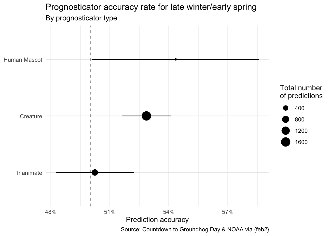
Your turn (time permitting): Make any other changes you would like to improve it.
# add your code heresessioninfo::session_info()─ Session info ───────────────────────────────────────────────────────────────
setting value
version R version 4.5.2 (2025-10-31)
os macOS Tahoe 26.3.1
system aarch64, darwin20
ui X11
language (EN)
collate en_US.UTF-8
ctype en_US.UTF-8
tz America/New_York
date 2026-03-13
pandoc 3.6.3 @ /Applications/Positron.app/Contents/Resources/app/quarto/bin/tools/aarch64/ (via rmarkdown)
quarto 1.9.33 @ /Applications/quarto/bin/quarto
─ Packages ───────────────────────────────────────────────────────────────────
! package * version date (UTC) lib source
P cli 3.6.5 2025-04-23 [?] RSPM (R 4.5.0)
P digest 0.6.39 2025-11-19 [?] RSPM (R 4.5.0)
P dplyr * 1.1.4 2023-11-17 [?] RSPM (R 4.5.0)
P evaluate 1.0.5 2025-08-27 [?] RSPM (R 4.5.0)
P farver 2.1.2 2024-05-13 [?] RSPM (R 4.5.0)
P fastmap 1.2.0 2024-05-15 [?] RSPM (R 4.5.0)
P feb2 * 0.2.1 2026-02-03 [?] Github (ericpgreen/feb2@05c3753)
P forcats * 1.0.1 2025-09-25 [?] RSPM (R 4.5.0)
P generics 0.1.4 2025-05-09 [?] RSPM (R 4.5.0)
P ggplot2 * 4.0.1 2025-11-14 [?] RSPM (R 4.5.0)
P glue 1.8.0 2024-09-30 [?] RSPM (R 4.5.0)
P gtable 0.3.6 2024-10-25 [?] RSPM (R 4.5.0)
P here 1.0.2 2025-09-15 [?] CRAN (R 4.5.0)
P hms 1.1.4 2025-10-17 [?] RSPM (R 4.5.0)
P htmltools 0.5.9 2025-12-04 [?] RSPM (R 4.5.0)
P htmlwidgets 1.6.4 2023-12-06 [?] RSPM (R 4.5.0)
P jsonlite 2.0.0 2025-03-27 [?] RSPM (R 4.5.0)
P knitr 1.51 2025-12-20 [?] RSPM (R 4.5.0)
P labeling 0.4.3 2023-08-29 [?] RSPM (R 4.5.0)
P lifecycle 1.0.4 2023-11-07 [?] RSPM (R 4.5.0)
P lubridate * 1.9.4 2024-12-08 [?] RSPM (R 4.5.0)
P magrittr 2.0.4 2025-09-12 [?] RSPM (R 4.5.0)
P otel 0.2.0 2025-08-29 [?] RSPM (R 4.5.0)
P pillar 1.11.1 2025-09-17 [?] RSPM (R 4.5.0)
P pkgconfig 2.0.3 2019-09-22 [?] RSPM (R 4.5.0)
P purrr * 1.2.0 2025-11-04 [?] CRAN (R 4.5.0)
P R6 2.6.1 2025-02-15 [?] RSPM (R 4.5.0)
P ragg 1.5.0 2025-09-02 [?] RSPM (R 4.5.0)
P RColorBrewer 1.1-3 2022-04-03 [?] RSPM (R 4.5.0)
P readr * 2.1.6 2025-11-14 [?] RSPM (R 4.5.0)
renv 1.1.5 2025-07-24 [1] RSPM (R 4.5.0)
P rlang 1.1.6 2025-04-11 [?] RSPM (R 4.5.0)
P rmarkdown 2.30 2025-09-28 [?] RSPM (R 4.5.0)
P rprojroot 2.1.1 2025-08-26 [?] RSPM (R 4.5.0)
P S7 0.2.1 2025-11-14 [?] RSPM (R 4.5.0)
P scales * 1.4.0 2025-04-24 [?] RSPM (R 4.5.0)
P sessioninfo 1.2.3 2025-02-05 [?] RSPM (R 4.5.0)
P stringi 1.8.7 2025-03-27 [?] RSPM (R 4.5.0)
P stringr * 1.6.0 2025-11-04 [?] RSPM (R 4.5.0)
P systemfonts 1.3.1 2025-10-01 [?] RSPM (R 4.5.0)
P textshaping 1.0.4 2025-10-10 [?] RSPM (R 4.5.0)
P tibble * 3.3.0 2025-06-08 [?] RSPM (R 4.5.0)
P tidyr * 1.3.2 2025-12-19 [?] RSPM (R 4.5.0)
P tidyselect 1.2.1 2024-03-11 [?] RSPM (R 4.5.0)
P tidyverse * 2.0.0 2023-02-22 [?] RSPM (R 4.5.0)
P timechange 0.3.0 2024-01-18 [?] RSPM (R 4.5.0)
P tzdb 0.5.0 2025-03-15 [?] RSPM (R 4.5.0)
P utf8 1.2.6 2025-06-08 [?] RSPM (R 4.5.0)
P vctrs 0.6.5 2023-12-01 [?] RSPM (R 4.5.0)
P withr 3.0.2 2024-10-28 [?] RSPM (R 4.5.0)
P xfun 0.55 2025-12-16 [?] CRAN (R 4.5.2)
P yaml 2.3.12 2025-12-10 [?] RSPM (R 4.5.0)
[1] /Users/bcs88/Projects/info-2950/course-site/renv/library/macos/R-4.5/aarch64-apple-darwin20
[2] /Users/bcs88/Library/Caches/org.R-project.R/R/renv/sandbox/macos/R-4.5/aarch64-apple-darwin20/4cd76b74
* ── Packages attached to the search path.
P ── Loaded and on-disk path mismatch.
──────────────────────────────────────────────────────────────────────────────