Linear regression with a single predictor

Lecture 18

Dr. Benjamin Soltoff

Cornell University
INFO 2951 - Spring 2025

March 25, 2025

Announcements

Announcements

• Homework 06
• Project EDA
• Extra credit

Modeling

Modeling

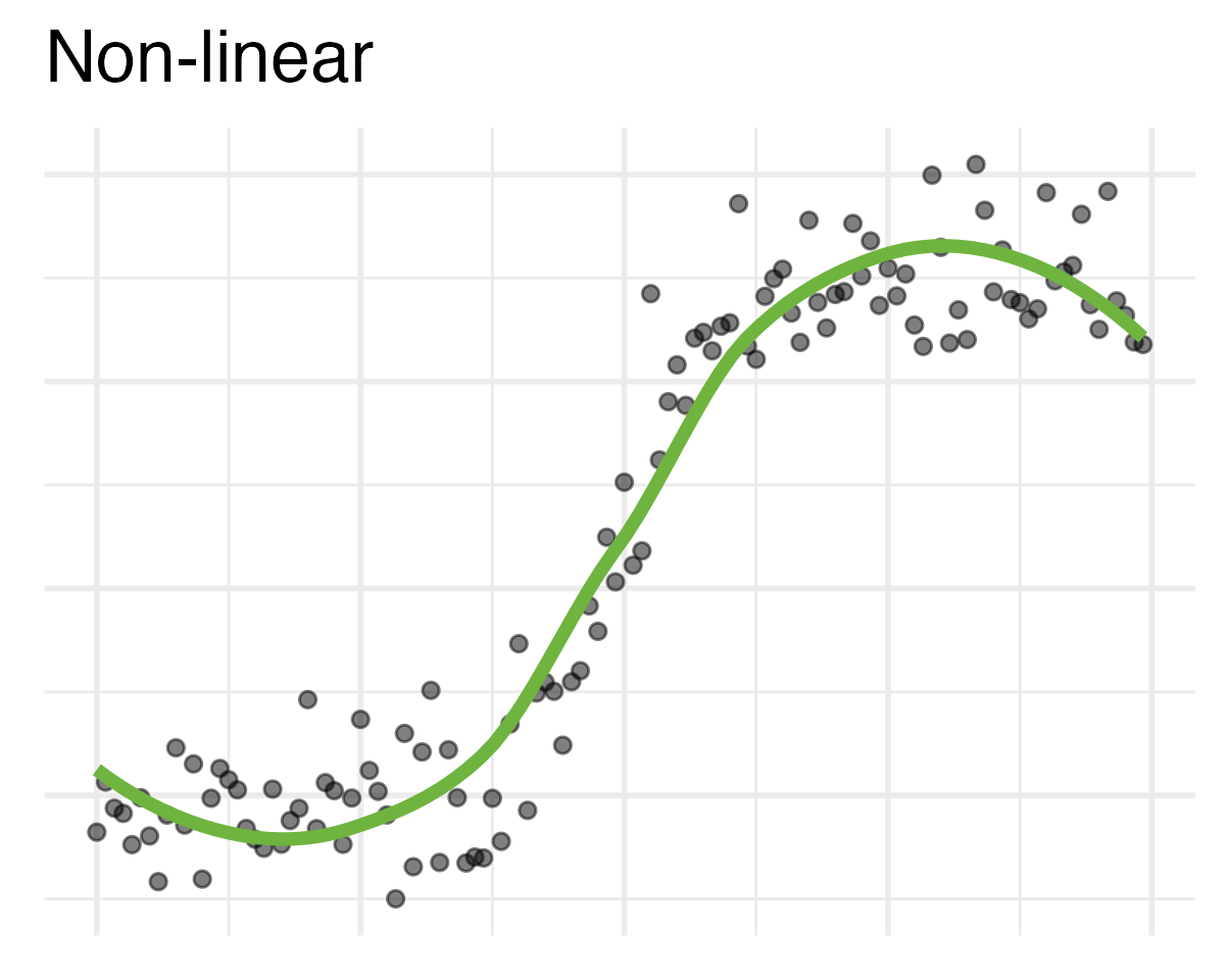
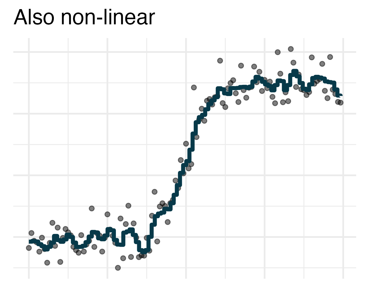
• Use models to explain the relationship between variables and to make predictions
• Many different types of models
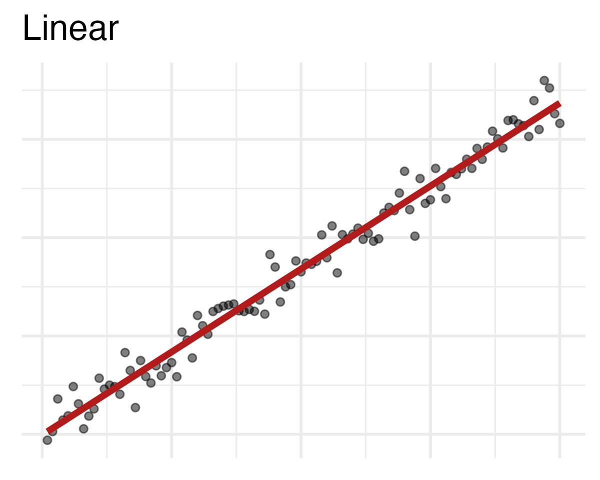
  • Linear models – classic forms used for statistical inference
  • Nonlinear models – much more common in machine learning for prediction

Modeling vocabulary

• Predictor/feature/explanatory variable/independent variable
• Outcome/dependent variable/response variable
• Correlation
• Regression line (for linear models)
  • Slope
  • Intercept

Data overview

# A tibble: 146 × 3
   film                    critics audience
   <chr>                     <int>    <int>
 1 Avengers: Age of Ultron      74       86
 2 Cinderella                   85       80
 3 Ant-Man                      80       90
 4 Do You Believe?              18       84
 5 Hot Tub Time Machine 2       14       28
 6 The Water Diviner            63       62
 7 Irrational Man               42       53
 8 Top Five                     86       64
 9 Shaun the Sheep Movie        99       82
10 Love & Mercy                 89       87
# ℹ 136 more rows

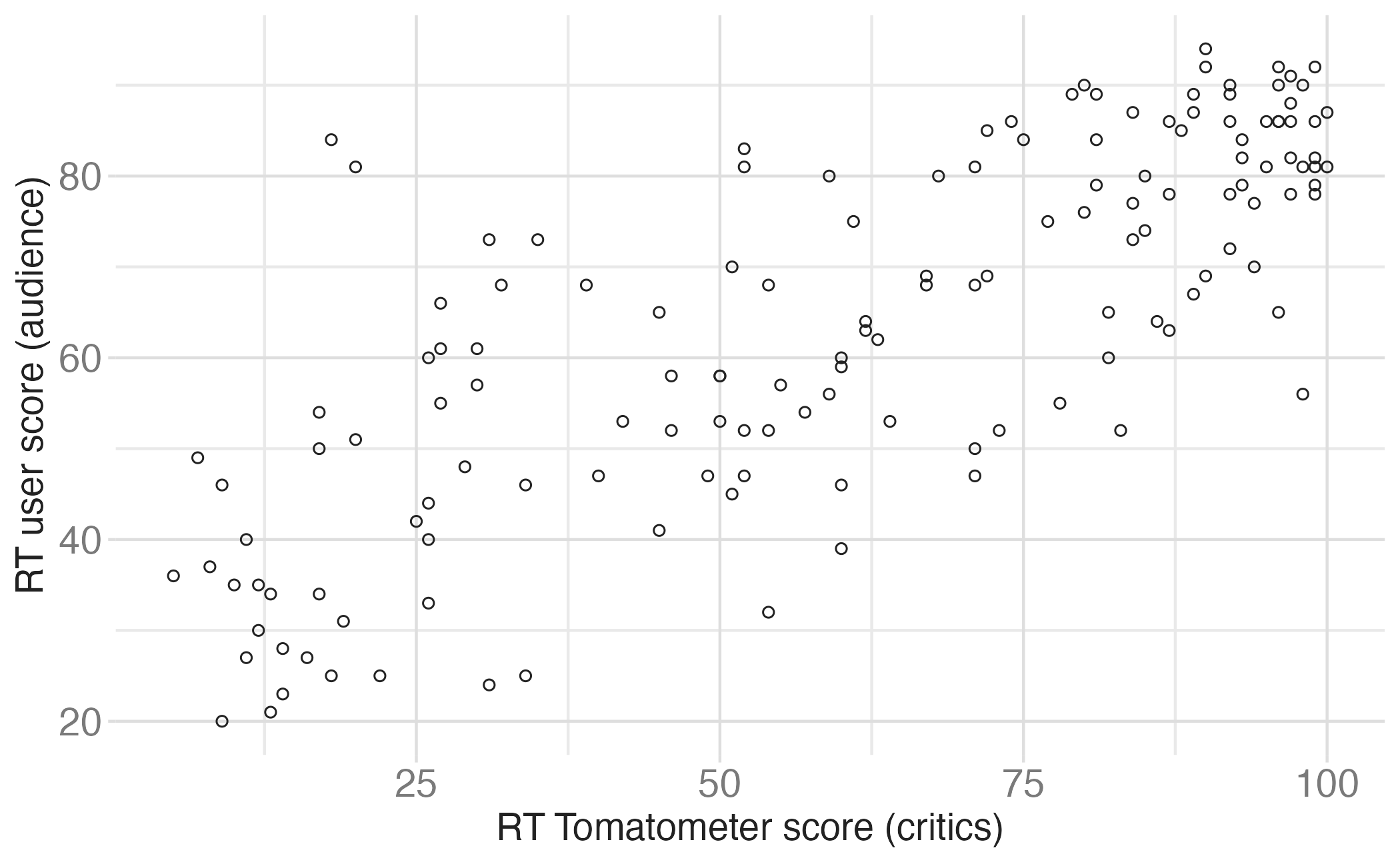
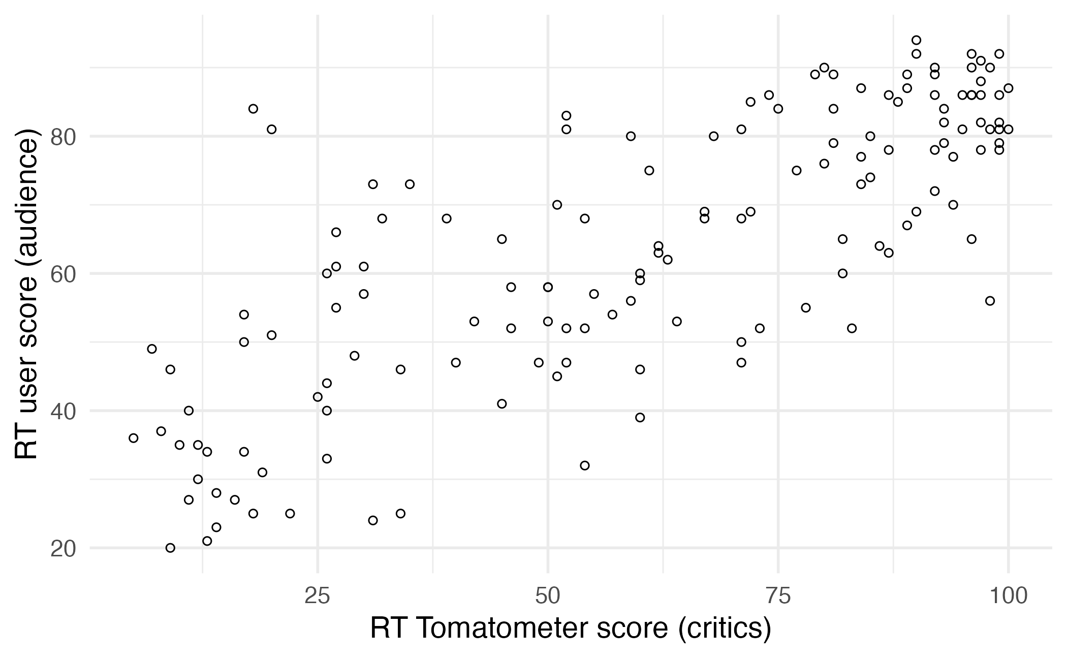
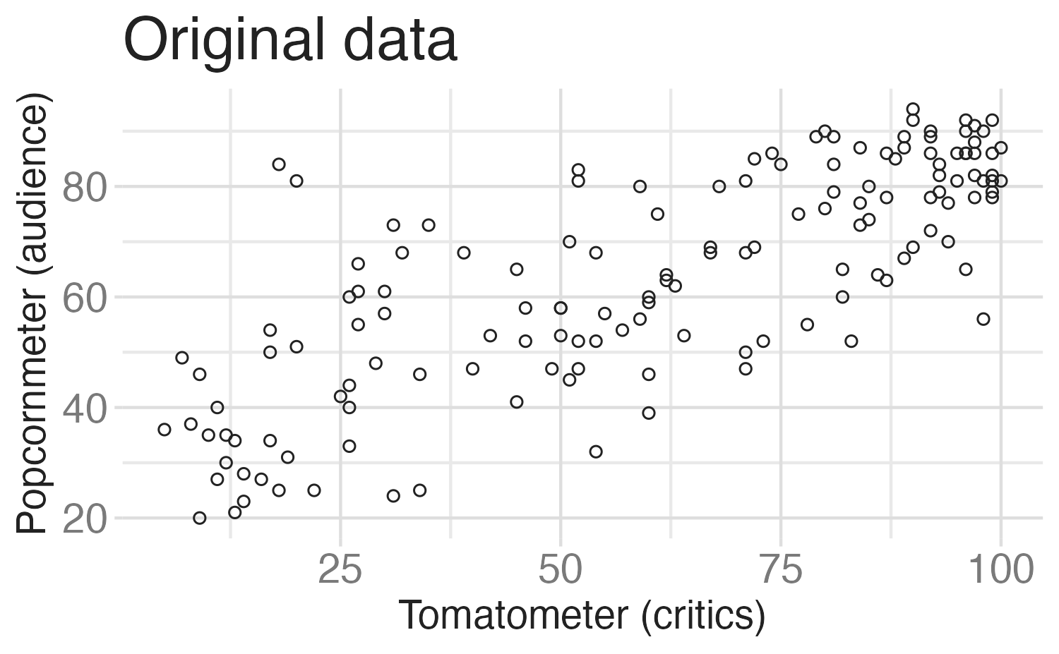
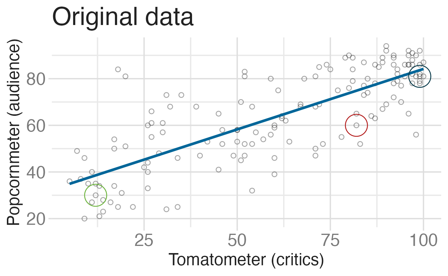
Modeling film ratings

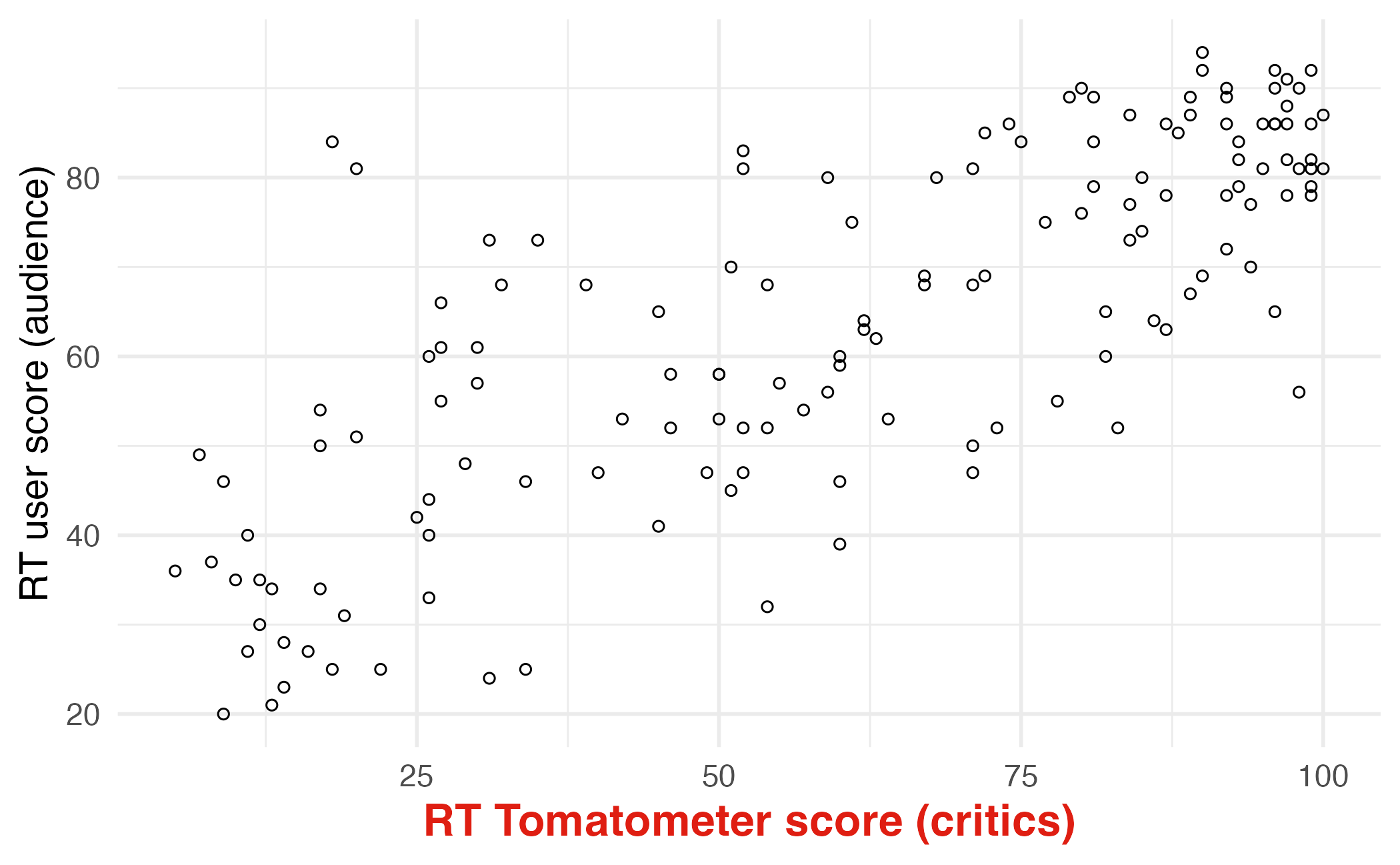
• What is the relationship between the critics and audience scores for films?
• What is your best guess for a film’s audience score if the critics rated it a 73?

Predictor (explanatory variable)

audience	critics
86	74
80	85
90	80
84	18
28	14
62	63
...	...

Outcome (response variable)

audience	critics
86	74
80	85
90	80
84	18
28	14
62	63
...	...

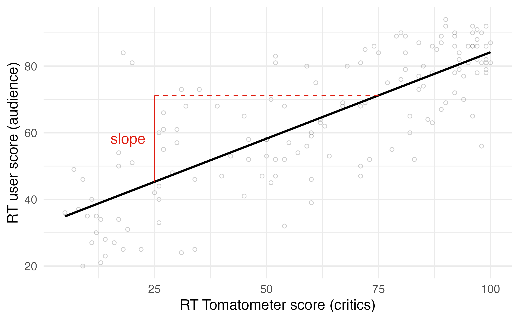
Regression line

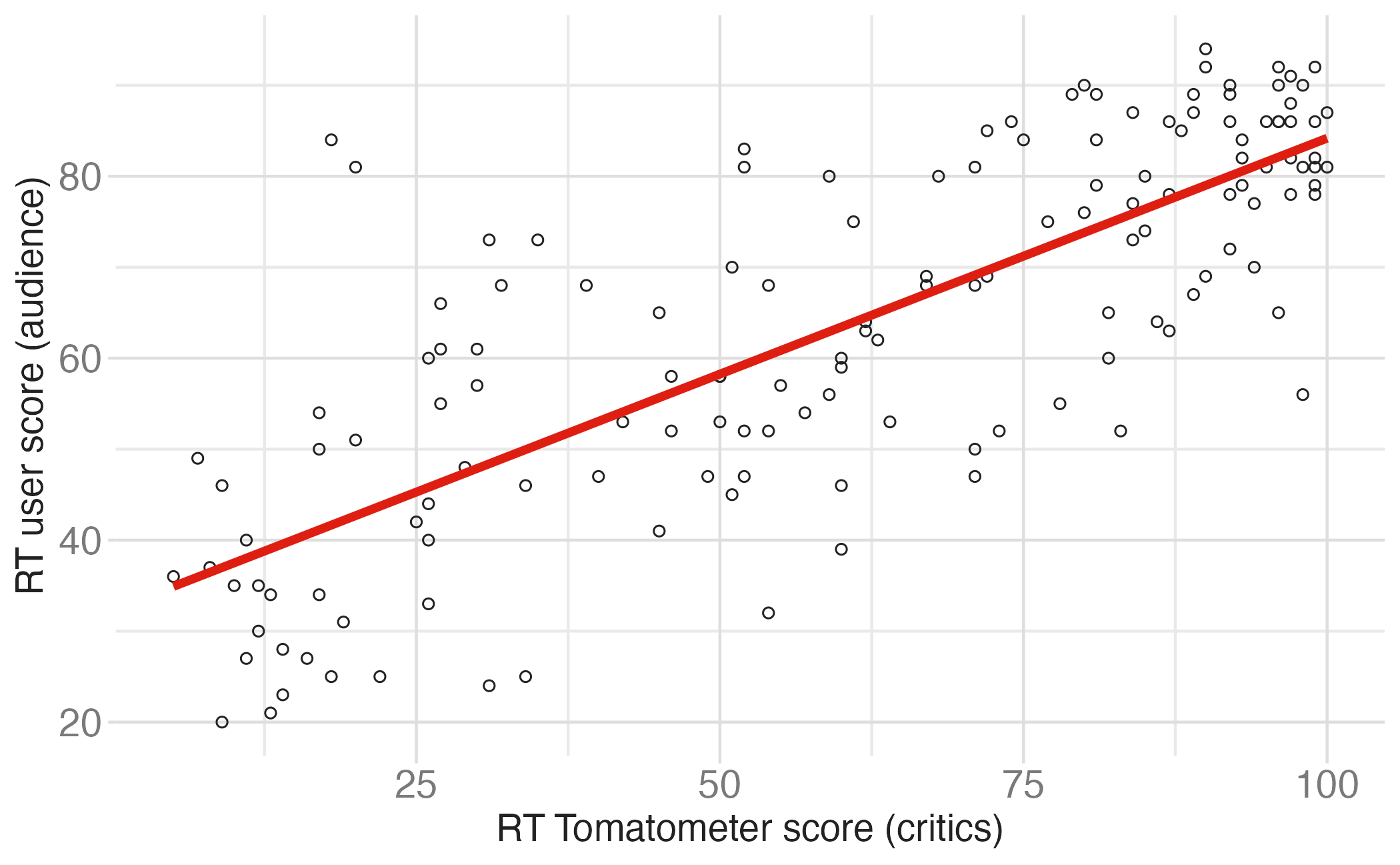
Regression line: slope

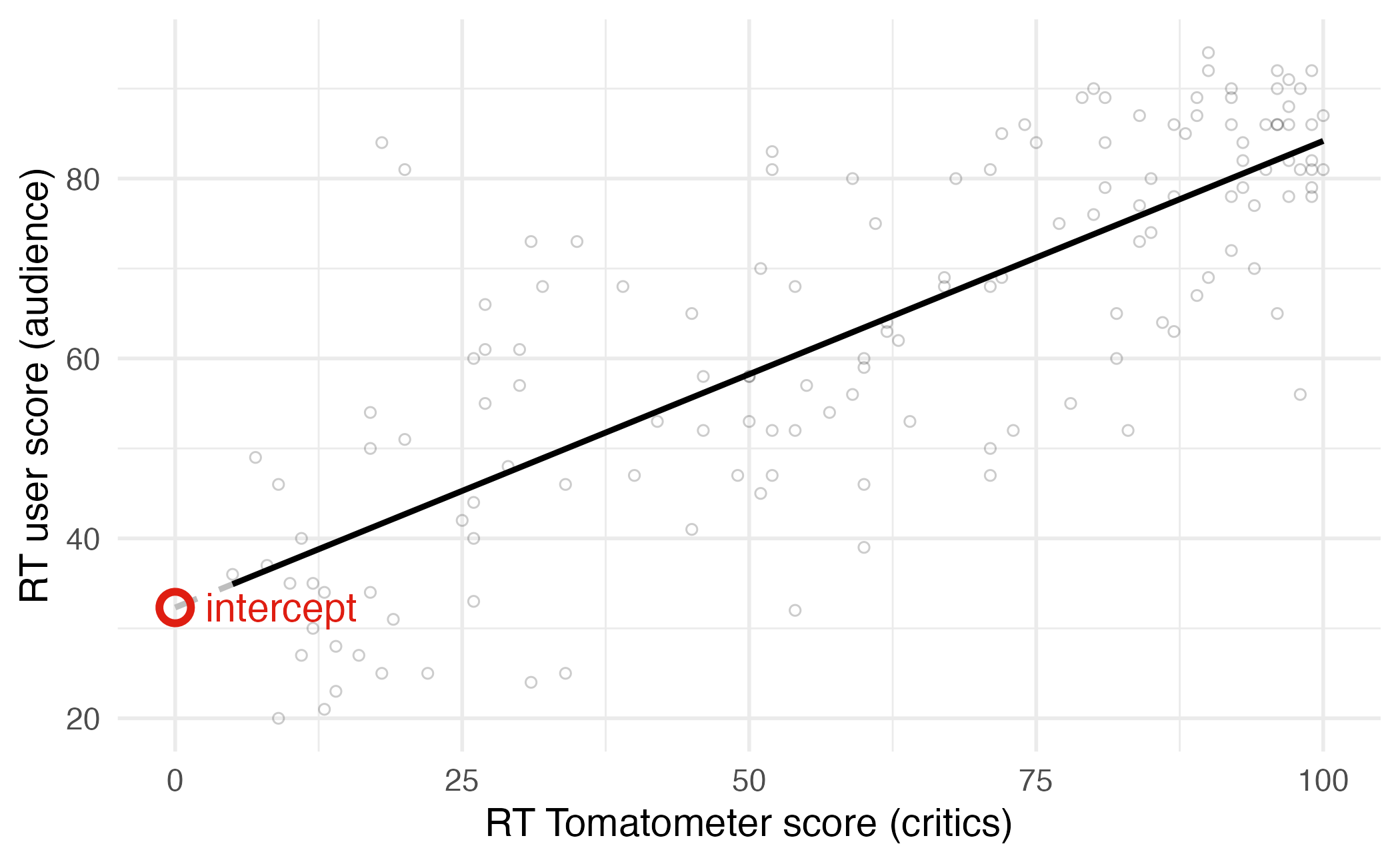
Regression line: intercept

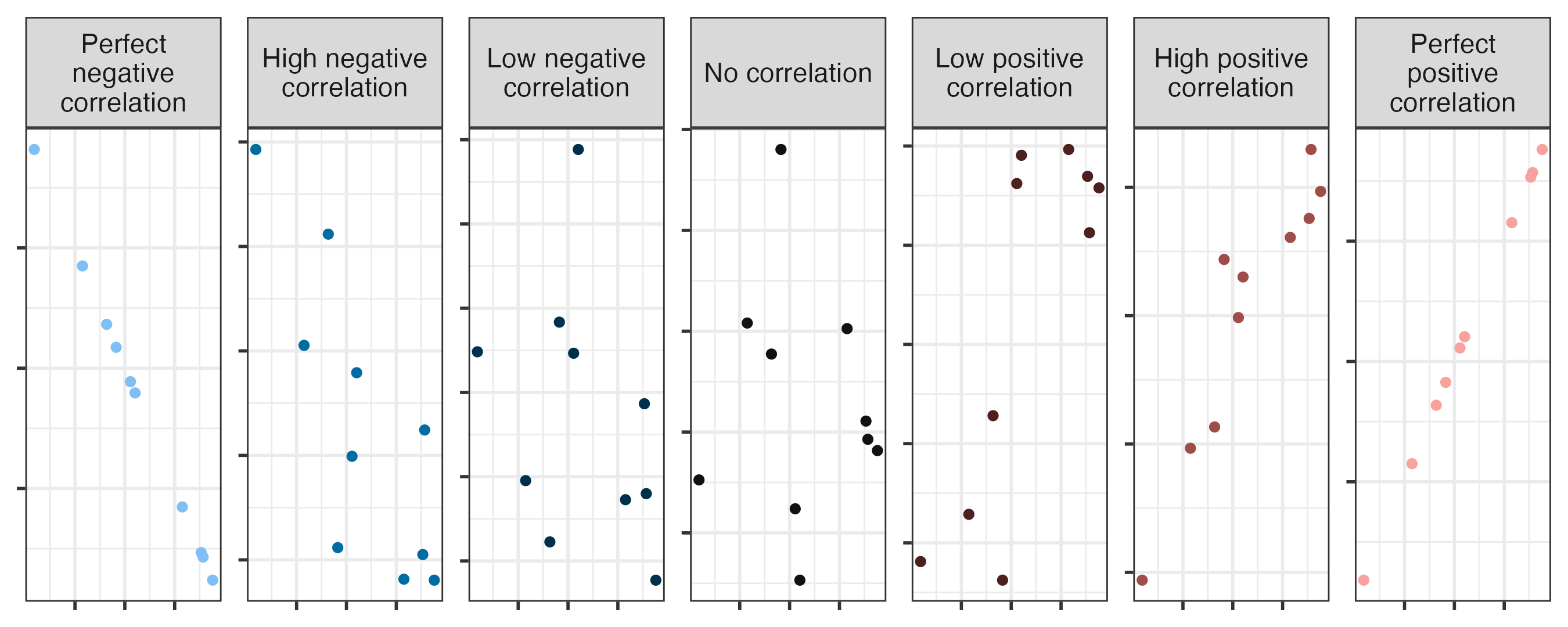
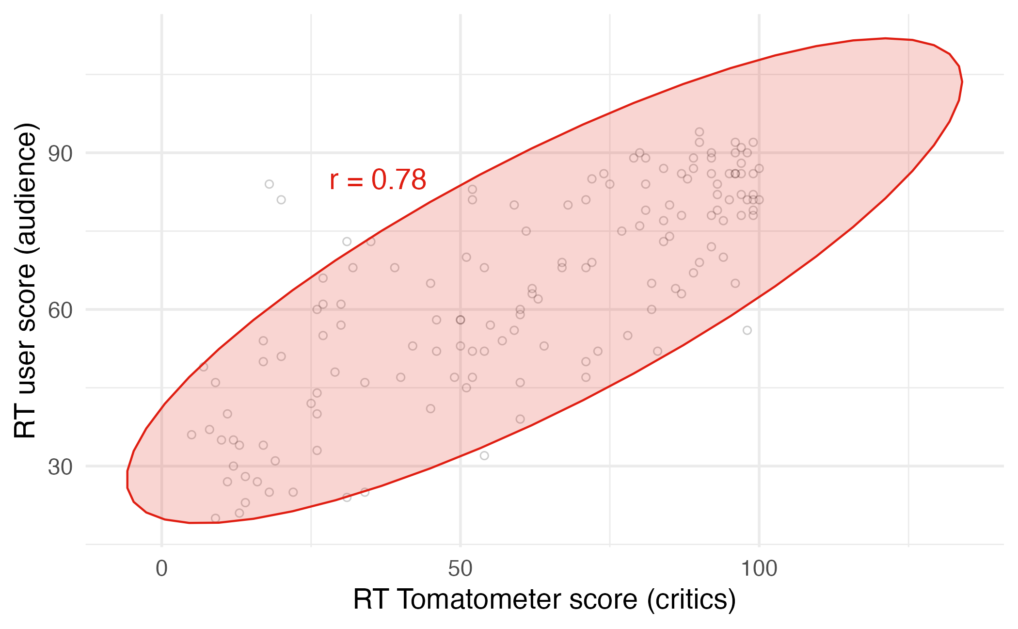
Correlation

Correlation

• Ranges between -1 and 1.
• Same sign as the slope.

Models with a single predictor

Regression model

A regression model is a function that describes the relationship between the outcome, \(Y\), and the predictor, \(X\).

\[ \begin{aligned} Y &= \color{black}{\textbf{Model}} + \text{Error} \\ &= \color{black}{\mathbf{f(X)}} + \epsilon \end{aligned} \]

Regression model

\[ \begin{aligned} Y &= \color{#DF1E12}{\textbf{Model}} + \text{Error} \\ &= \color{#DF1E12}{\mathbf{f(X)}} + \epsilon \end{aligned} \]

Simple linear regression

Use simple linear regression to model the relationship between a quantitative outcome (\(Y\)) and a single quantitative predictor (\(X\)):

\[ \begin{aligned} Y &= f(X) \\ &= \beta_0 + \beta_1 X + \epsilon \end{aligned} \]

• \(\beta_1\): True slope of the relationship between \(X\) and \(Y\)
• \(\beta_0\): True intercept of the relationship between \(X\) and \(Y\)
• \(\epsilon\): Error (residual)

But we don’t know \(\beta_0\) and \(\beta_1\) - we only have a sample of 146 movies!

Simple linear regression

\[\Large{\hat{Y} = b_0 + b_1 X}\]

• \(b_1\): Estimated slope of the relationship between \(X\) and \(Y\)
• \(b_0\): Estimated intercept of the relationship between \(X\) and \(Y\)
• No error term!

• How do we choose values for \(b_1\) and \(b_0\)?

Choosing values for \(b_1\) and \(b_0\)

#| '!! shinylive warning !!': |
#|   shinylive does not work in self-contained HTML documents.
#|   Please set `embed-resources: false` in your metadata.
#| label: lm-values
#| viewerHeight: 700
#| viewerWidth: "100%"
#| standalone: true

library(shiny)
library(ggplot2)
library(fivethirtyeight)
library(bslib)
library(dplyr)

# Create movie_scores from fandango dataset
movie_scores <- fandango %>%
  rename(
    critics = rottentomatoes,
    audience = rottentomatoes_user
  )

# Calculate actual regression line parameters
actual_model <- lm(audience ~ critics, data = movie_scores)
actual_intercept <- coef(actual_model)[1]
actual_slope <- coef(actual_model)[2]

# Set default values slightly off from actual values
default_intercept <- round(actual_intercept + 10) # Add 10 to be "slightly wrong"
default_slope <- round(actual_slope - 0.2, 2) # Subtract 0.2 to be "slightly wrong"

ui <- page_sidebar(
  # title = "Linear Regression: Movie Scores Explorer",
  theme = bs_theme(
    version = 5,
    bootswatch = "default",
    base_font_size = "22px"  # Increased base font size
  ),
  
  # Left sidebar with inputs
  sidebar = sidebar(
    width = "35%",  # Increased width for more space
    tags$style(HTML("
      .irs-min, .irs-max, .irs-single, .irs-from, .irs-to, .irs-grid-text {
        font-size: 20px !important;
      }
      .irs-grid-pol {
        height: 6px !important;
      }
      .irs-bar, .irs-line {
        height: 12px !important;
      }
      .irs-handle {
        width: 24px !important;
        height: 24px !important;
        top: 26px !important;
      }
      .control-label {
        font-size: 24px !important;
        font-weight: bold !important;
        margin-bottom: 10px !important;
      }
    ")),
    
    sliderInput(
      "intercept", 
      "Intercept:", 
      min = 0, 
      max = 100,
      value = default_intercept, 
      step = 1,
      width = "100%"
    ),
    
    tags$div(style = "margin-top: 30px;"),  # Add spacing between sliders
    
    sliderInput(
      "slope", 
      "Slope:", 
      min = -2, 
      max = 2, 
      value = default_slope, 
      step = 0.05,
      width = "100%"
    )
  ),
  
  # Main panel with plot
  card(
    full_screen = TRUE,
    plotOutput("regressionPlot", height = "500px")
  )
)

server <- function(input, output) {
  
  # Create the plot
  output$regressionPlot <- renderPlot({
    # User defined regression line
    user_intercept <- input$intercept
    user_slope <- input$slope
    
    # Create simple plot
    ggplot(movie_scores, aes(x = critics, y = audience)) +
      geom_point(alpha = 0.7, size = 3) +  # Larger points
      geom_abline(intercept = user_intercept, slope = user_slope, 
                 color = "red", linewidth = 1.5) +  # Thicker line
      labs(
        x = "Critics Score",
        y = "Audience Score"
      ) +
      theme_minimal(base_size = 16) +  # Larger theme elements
      theme(
        axis.title = element_text(size = 18, face = "bold"),
        axis.text = element_text(size = 16)
      )
  })
}

shinyApp(ui = ui, server = server)

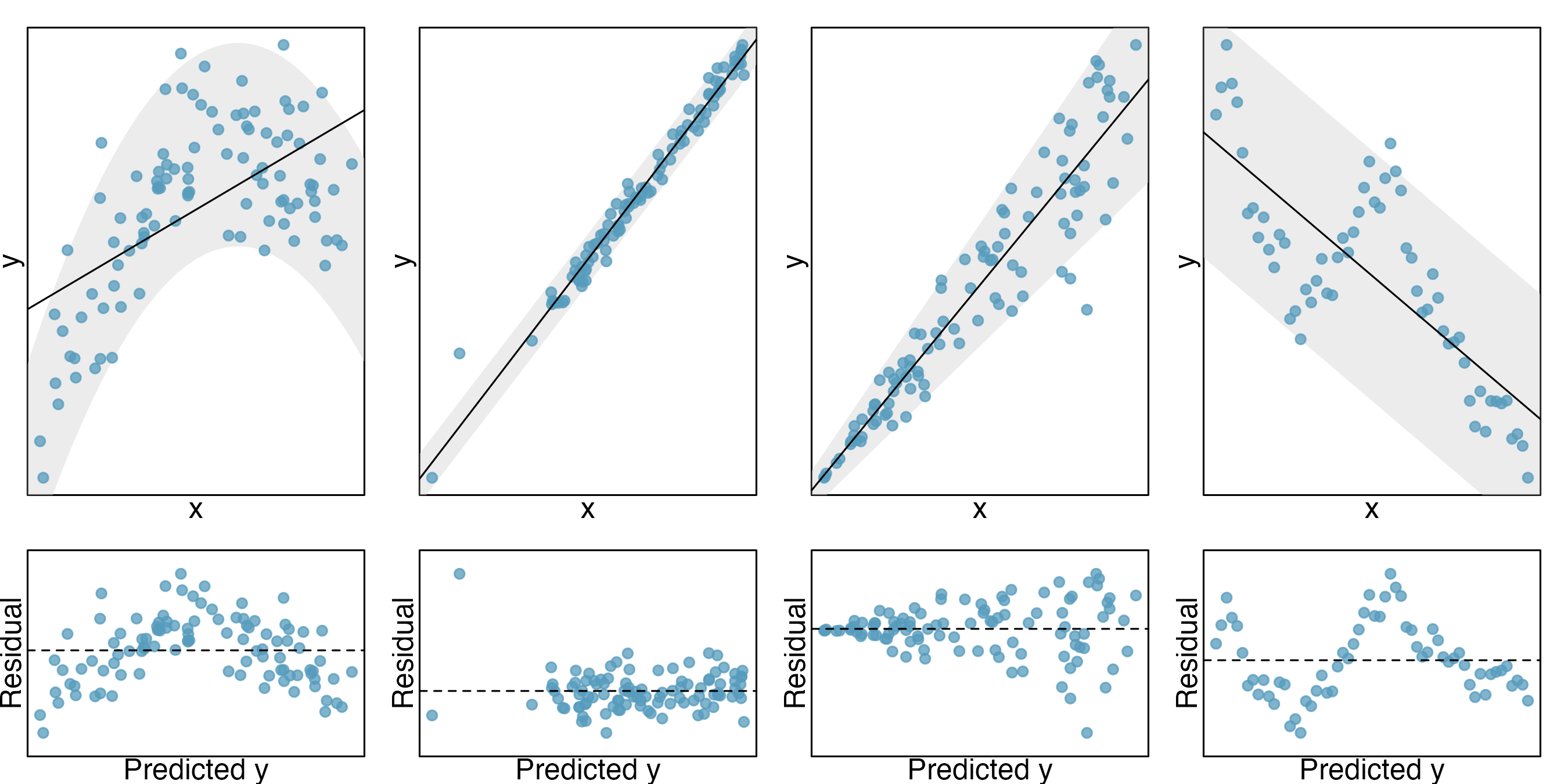
Residuals

\[\text{residual} = \text{observed} - \text{predicted} = y - \hat{y}\]

Least squares line

• The residual for the \(i^{th}\) observation is

\[e_i = \text{observed} - \text{predicted} = y_i - \hat{y}_i\]

• The sum of squared residuals is

\[e^2_1 + e^2_2 + \dots + e^2_n\]

• The least squares line is the one that minimizes the sum of squared residuals

Least squares line

movies_fit <- linear_reg() |>
  fit(audience ~ critics, data = movie_scores)

tidy(movies_fit)

# A tibble: 2 × 5
  term        estimate std.error statistic  p.value
  <chr>          <dbl>     <dbl>     <dbl>    <dbl>
1 (Intercept)   32.3      2.34        13.8 4.03e-28
2 critics        0.519    0.0345      15.0 2.70e-31

Slope and intercept

Properties of least squares regression

• The regression line goes through the center of mass point (the coordinates corresponding to average \(X\) and average \(Y\)): \(b_0 = \bar{Y} - b_1~\bar{X}\)

• Slope has the same sign as the correlation coefficient: \(b_1 = r \frac{sd_Y}{sd_X}\)

• Sum of the residuals is zero: \(\sum_{i = 1}^n \epsilon_i = 0\)

• Residuals and \(X\) values are uncorrelated

Interpreting the slope

The slope of the model for predicting audience score from critics score is 0.519. Which of the following is the best interpretation of this value?

1. For every one point increase in the critics score, the audience score goes up by 0.519 points, on average.
2. For every one point increase in the critics score, we expect the audience score to be higher by 0.519 points, on average.
3. For every one point increase in the critics score, the audience score goes up by 0.519 points.
4. For every one point increase in the audience score, the critics score goes up by 0.519 points, on average.

Interpreting slope & intercept

\[\widehat{\text{audience}} = 32.3 + 0.519 \times \text{critics}\]

• Slope: For every one point increase in the critics score, we expect the audience score to be higher by 0.519 points, on average.
• Intercept: If the critics score is 0 points, we expect the audience score to be 32.3 points.

Is the intercept meaningful?

✅ The intercept is meaningful in context of the data if

• the predictor can feasibly take values equal to or near zero or
• the predictor has values near zero in the observed data

🛑 Otherwise, it might not be meaningful!

Statistical inference with a single predictor

Birth weights and gestation time

Null hypothesis framework

Population of interest: All births in the United States

• \(H_0: \beta_1= 0\), there is no linear relationship between weight and weeks.
• \(H_A: \beta_1 \ne 0\), there is some linear relationship between weight and weeks.

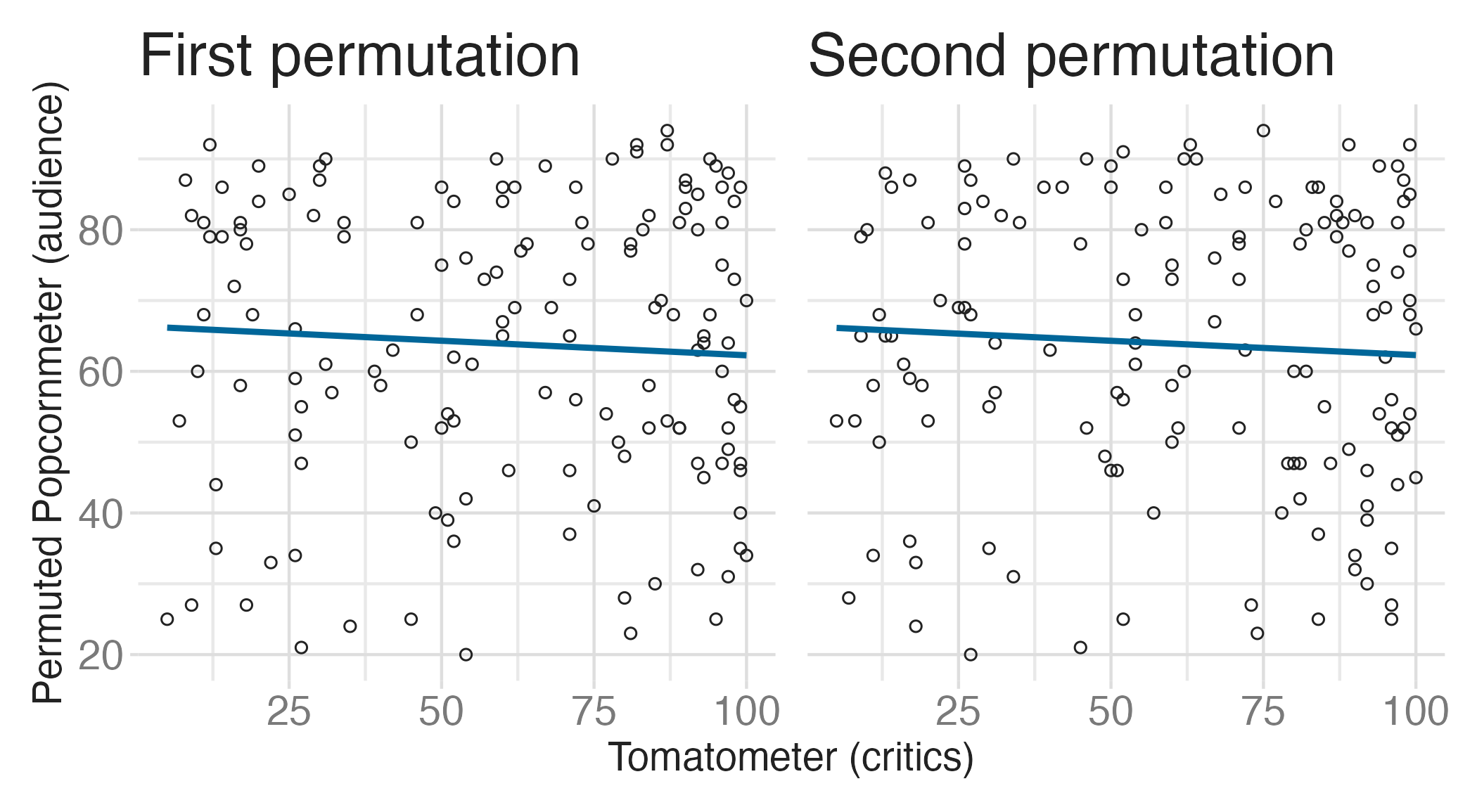
Permutation-based approach

Observed data

Characteristic	Beta	SE	Statistic	95% CI	p-value
(Intercept)	-5.7	1.61	-3.54	-8.9, -2.5	<0.001
weeks	0.34	0.042	8.07	0.25, 0.42	<0.001
Abbreviations: CI = Confidence Interval, SE = Standard Error

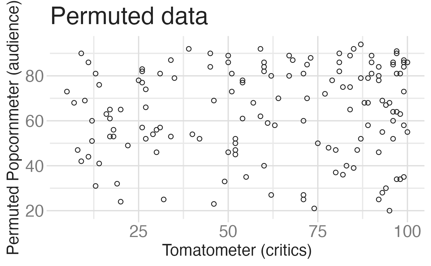
Variability of the statistic

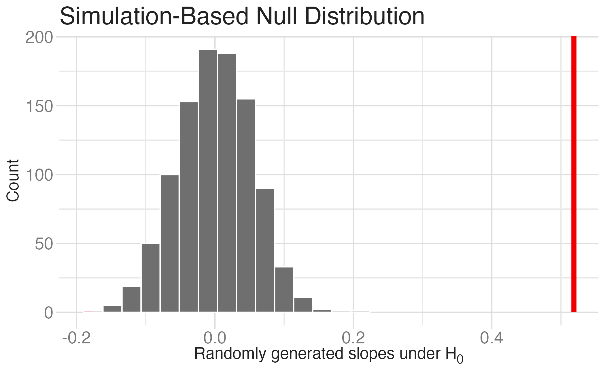
Observed statistic vs. null statistics

Bootstrap CI for the slope

Characteristic	Beta	SE	Statistic	95% CI	p-value
(Intercept)	6.2	0.708	8.79	4.8, 7.6	<0.001
mage	0.04	0.024	1.50	-0.01, 0.08	0.14
Abbreviations: CI = Confidence Interval, SE = Standard Error

Bootstrap resampling

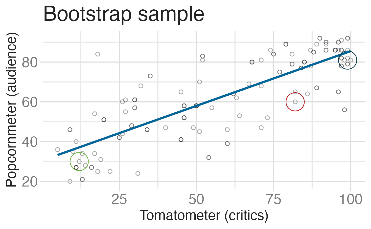
Bootstrap resampling (repeated)

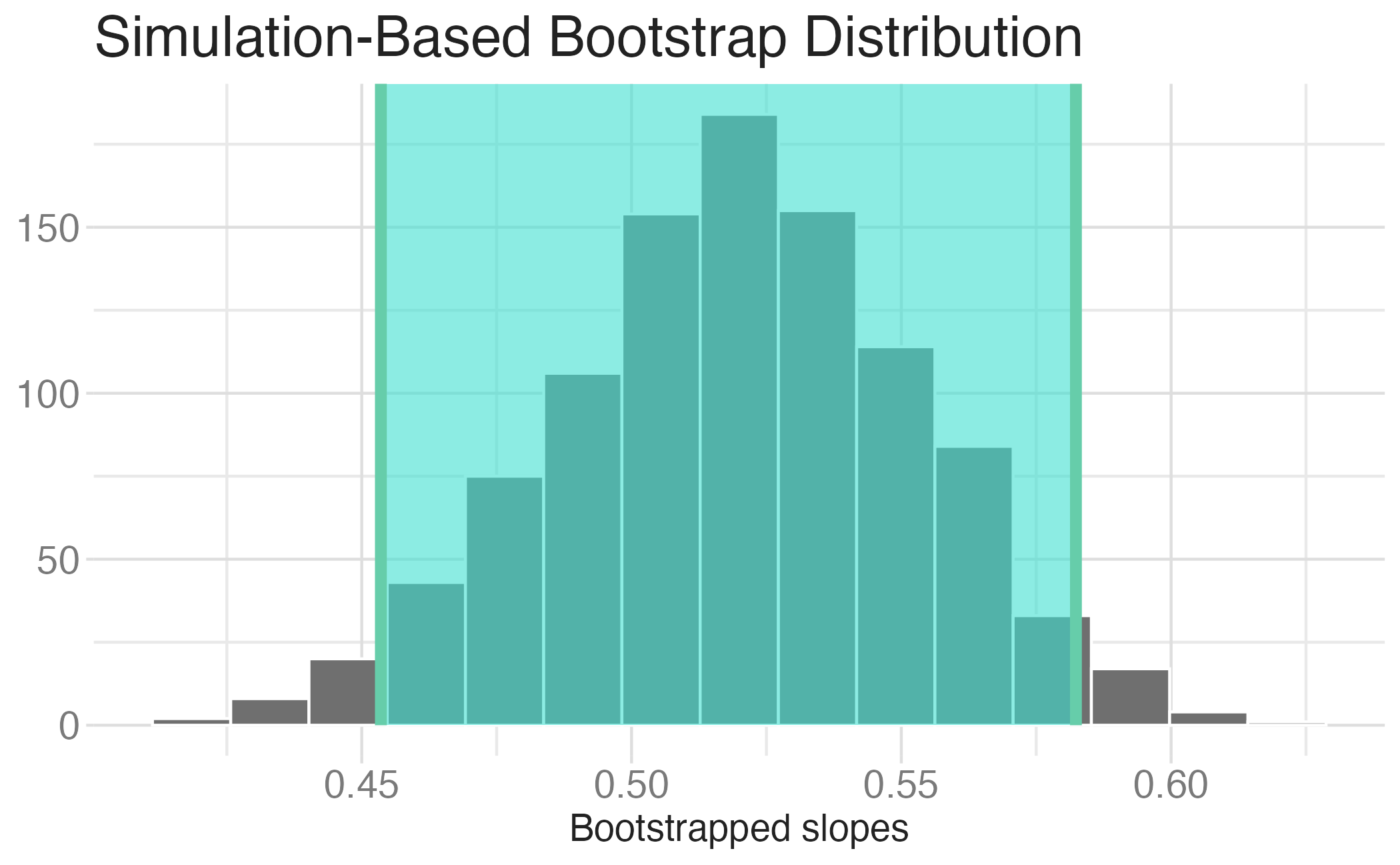
Bootstrap CI for the slope

Checking model conditions

• Linearity
• Independent observations
• Nearly normal residuals
• Constant or equal variability

Violations of model conditions

Application exercise

ae-16

Instructions

• Go to the course GitHub org and find your ae-16 (repo name will be suffixed with your GitHub name).
• Clone the repo in RStudio, run renv::restore() to install the required packages, open the Quarto document in the repo, and follow along and complete the exercises.
• Render, commit, and push your edits by the AE deadline – end of the day

Wrap up

Recap

• Linear regression fits a line to the relationship between \(X\) and \(Y\)
• It estimates coefficients that minimize the sum of squared error (residuals)
• We can use permutation tests and bootstrapping to make inferences about the coefficients
• Linear regression has specific assumptions that must be met in order to make valid inferences

Acknowledgments

• Draws upon material from Data Science in a Box licensed under Creative Commons Attribution-ShareAlike 4.0 International