
[1] 9 7 10 1 6 8 4 3 2 5 [1] 2 10 4 5 6 8 1 7 9 3 [1] 3 7 5 1 2 9 8 4 6 10Lecture 17
Cornell University
INFO 2951 - Spring 2026
March 19, 2026
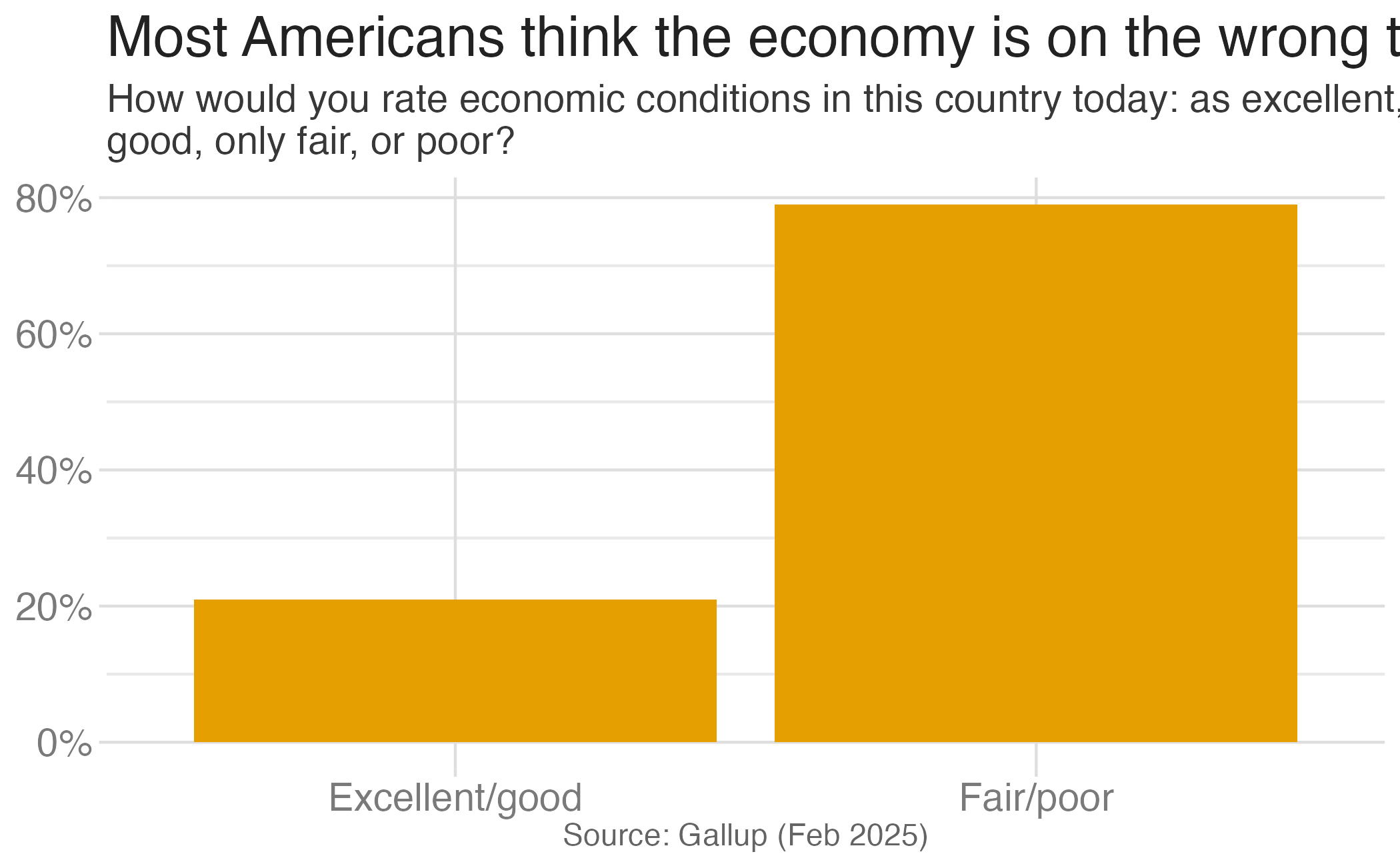
… is the process of using sample data to make conclusions about the underlying population from which the sample came
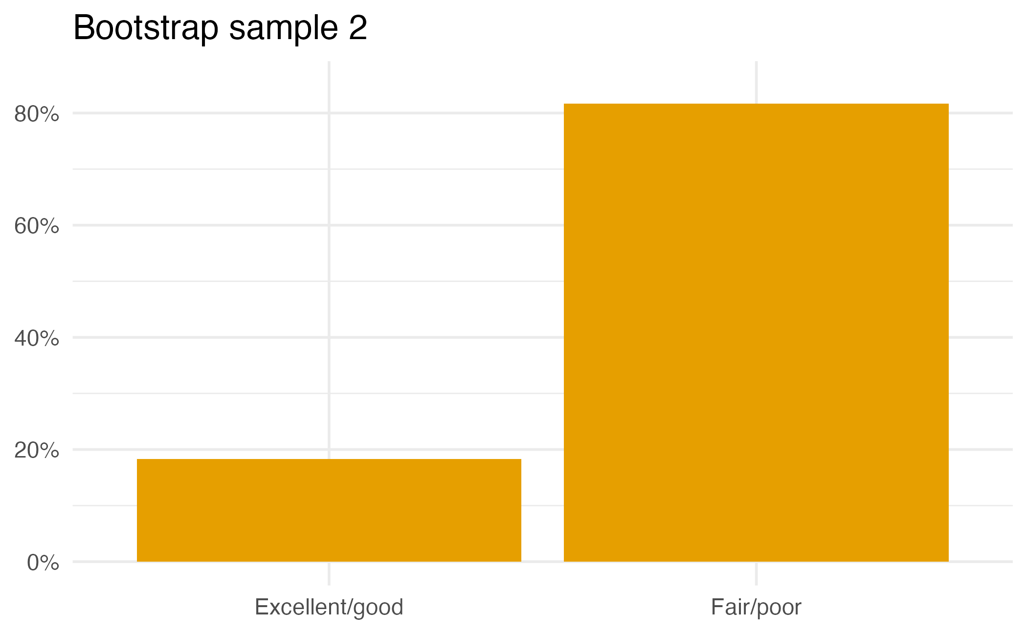
If you want to catch a fish, do you prefer a spear or a net?


If you want to estimate a population parameter, do you prefer to report a range of values the parameter might be in, or a single value?
A plausible range of values for the population parameter is a confidence interval.
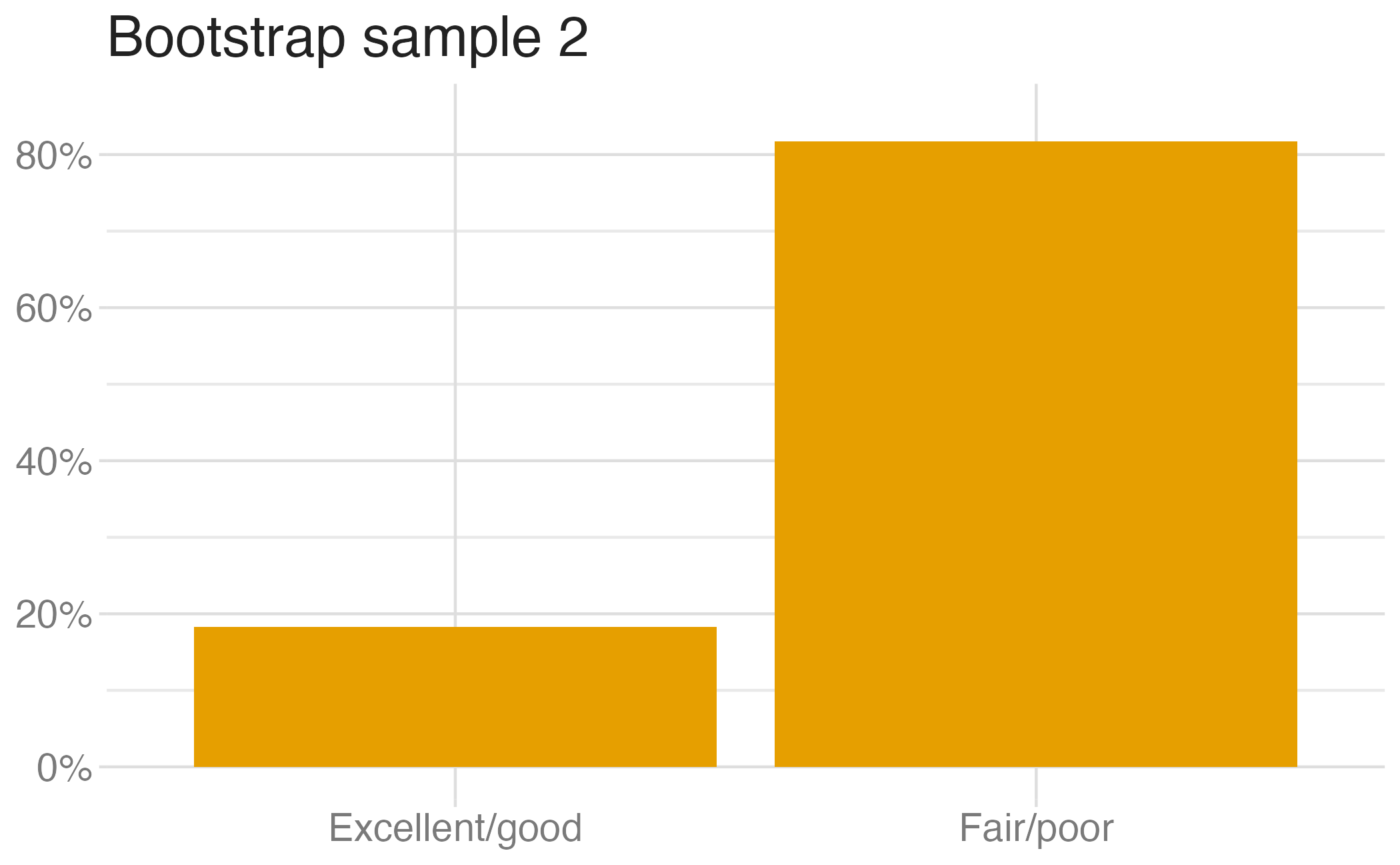
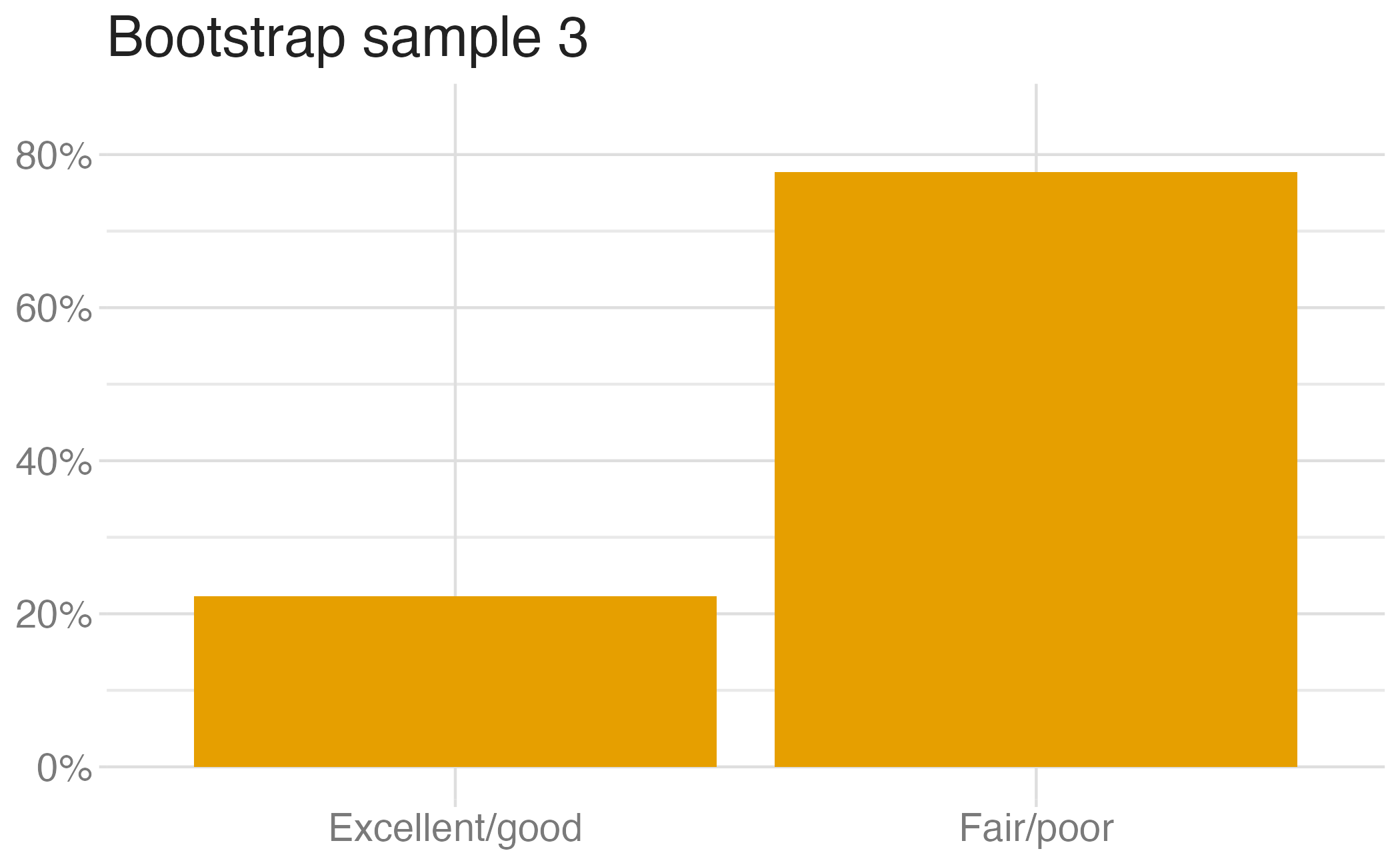
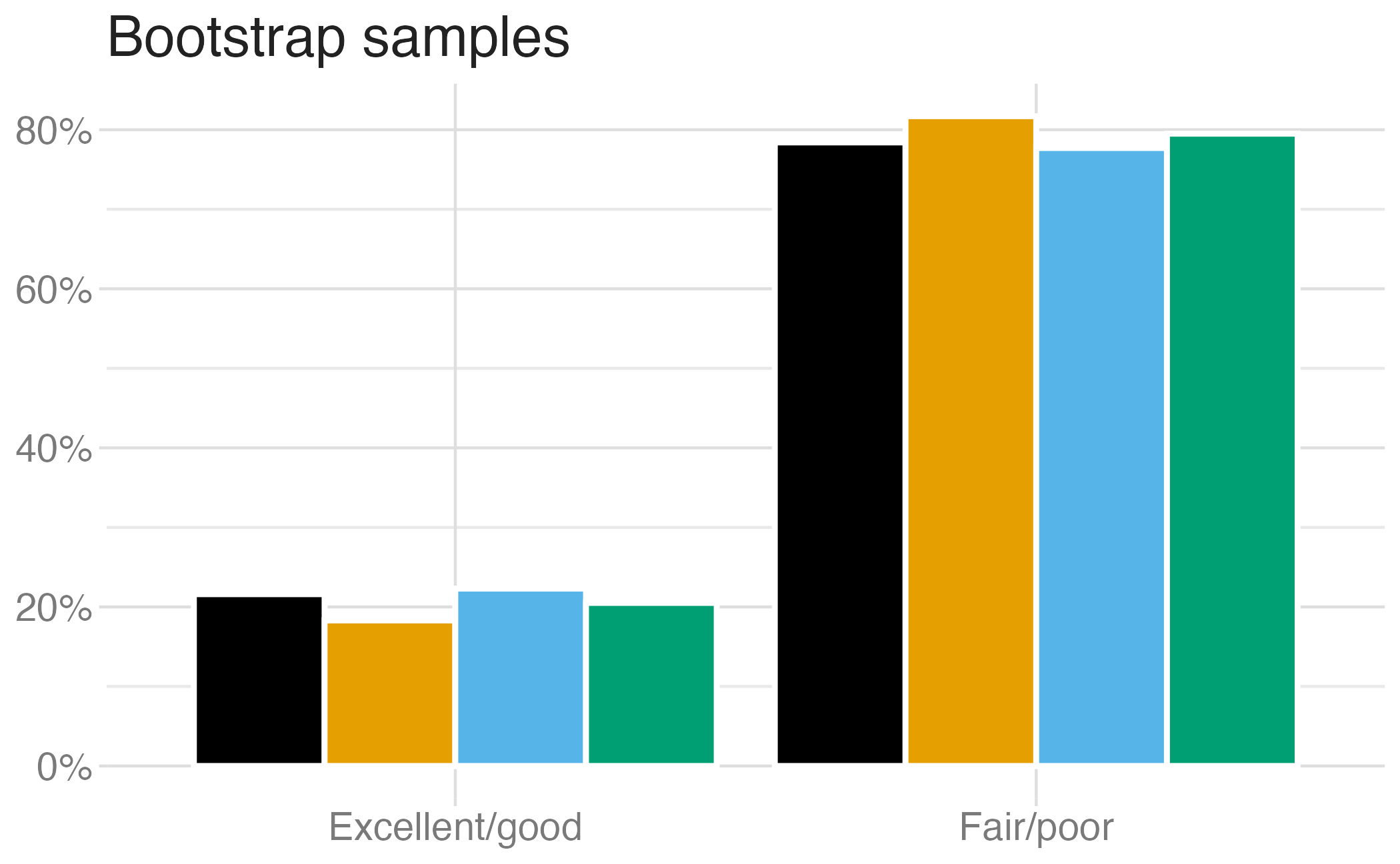
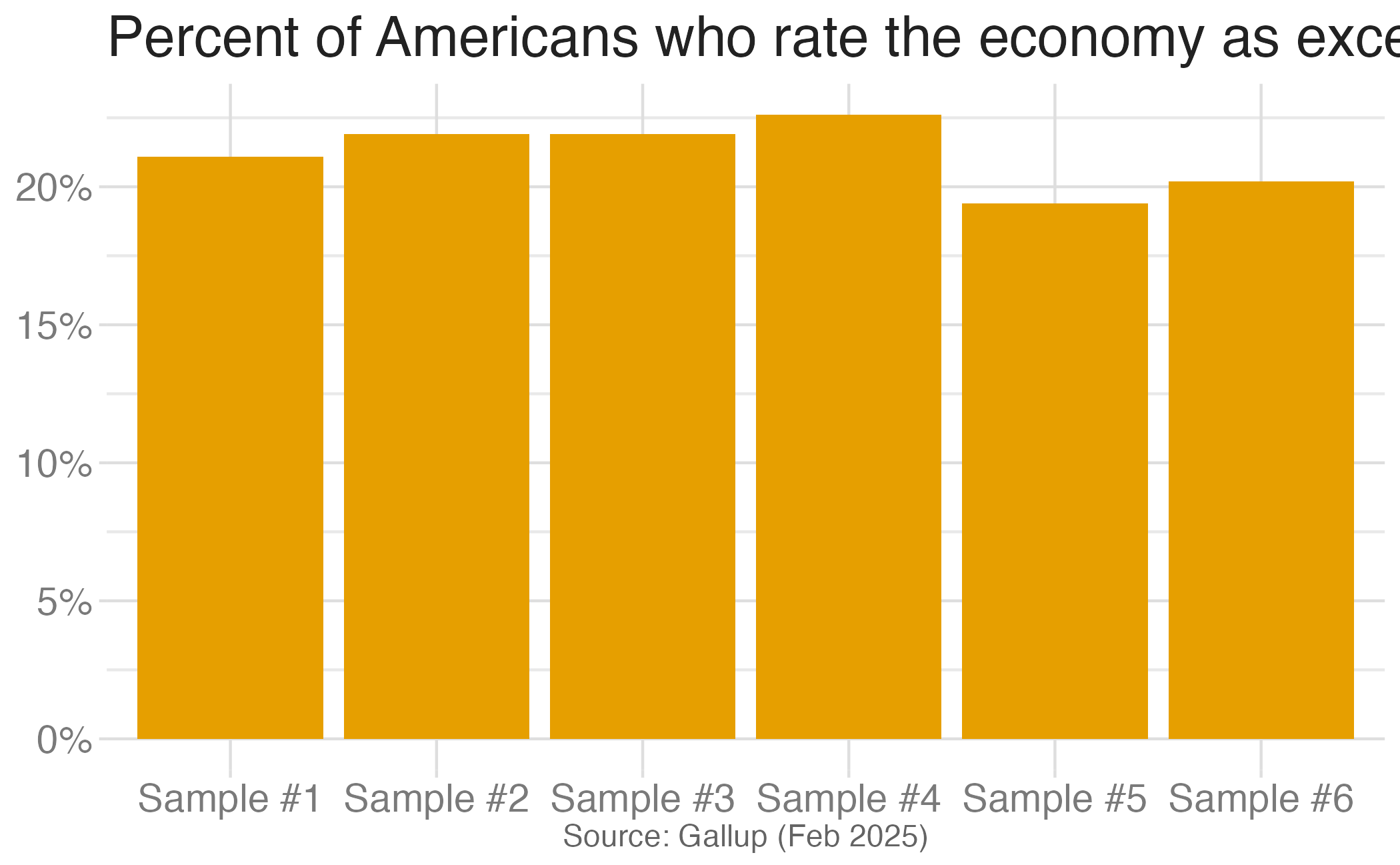
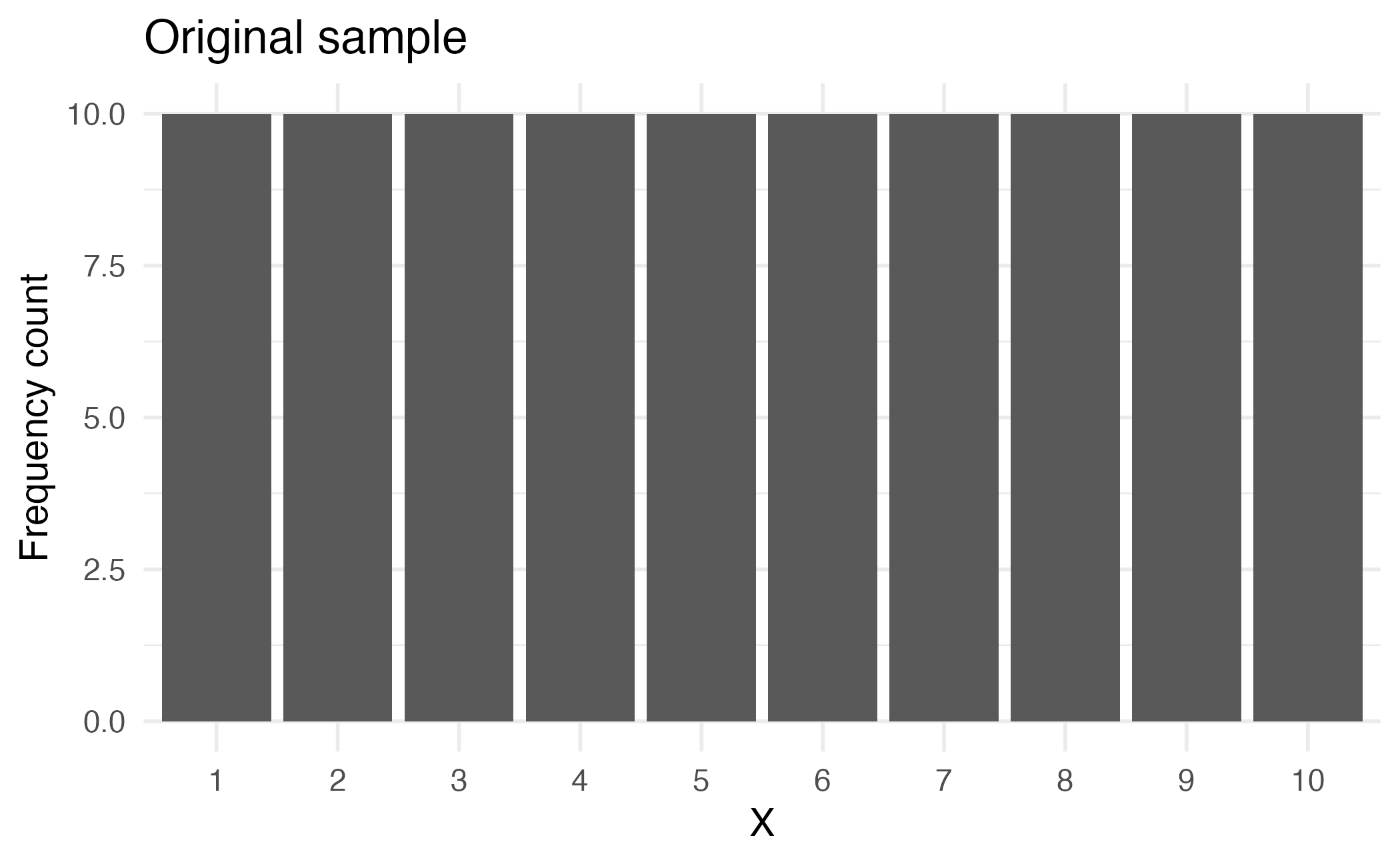
Suppose you randomly sample 50 students and 5 of them are left handed. If you were to take another random sample of 50 students, how many would you expect to be left handed? Would you be surprised if only 3 of them were left handed? Would you be surprised if 40 of them were left handed?
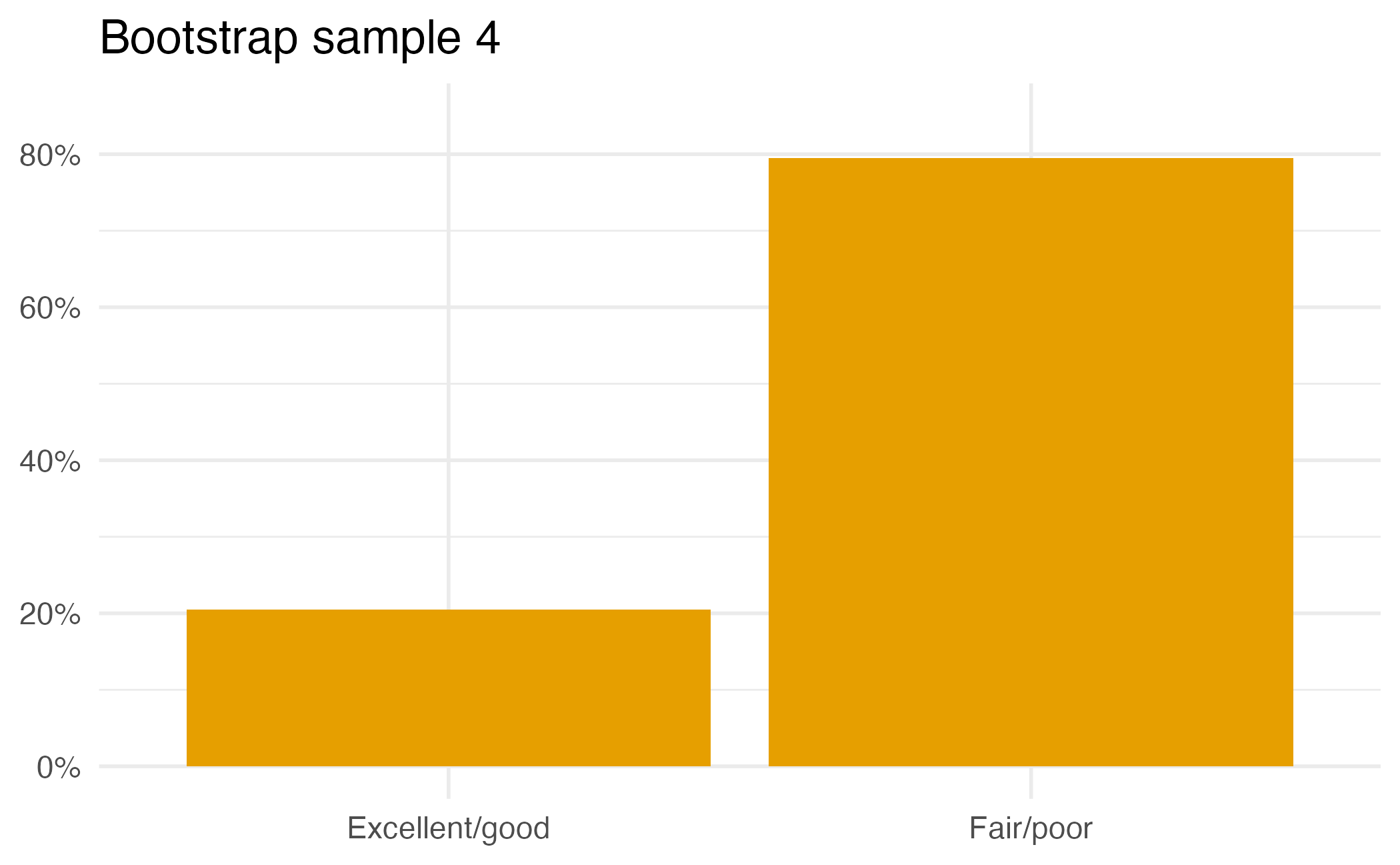
We can quantify the variability of sample statistics using
or
🥾
Data source: 🔗 Gallup
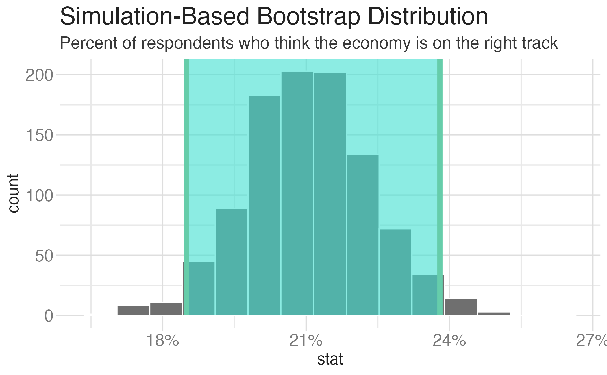
[1] 9 7 10 1 6 8 4 3 2 5 [1] 2 10 4 5 6 8 1 7 9 3 [1] 3 7 5 1 2 9 8 4 6 10# A tibble: 1 × 2
lower_ci upper_ci
<dbl> <dbl>
1 0.257 0.313We are 95% confident that the true proportion of Americans who think the economy is on the right track is between 26% and 31%.
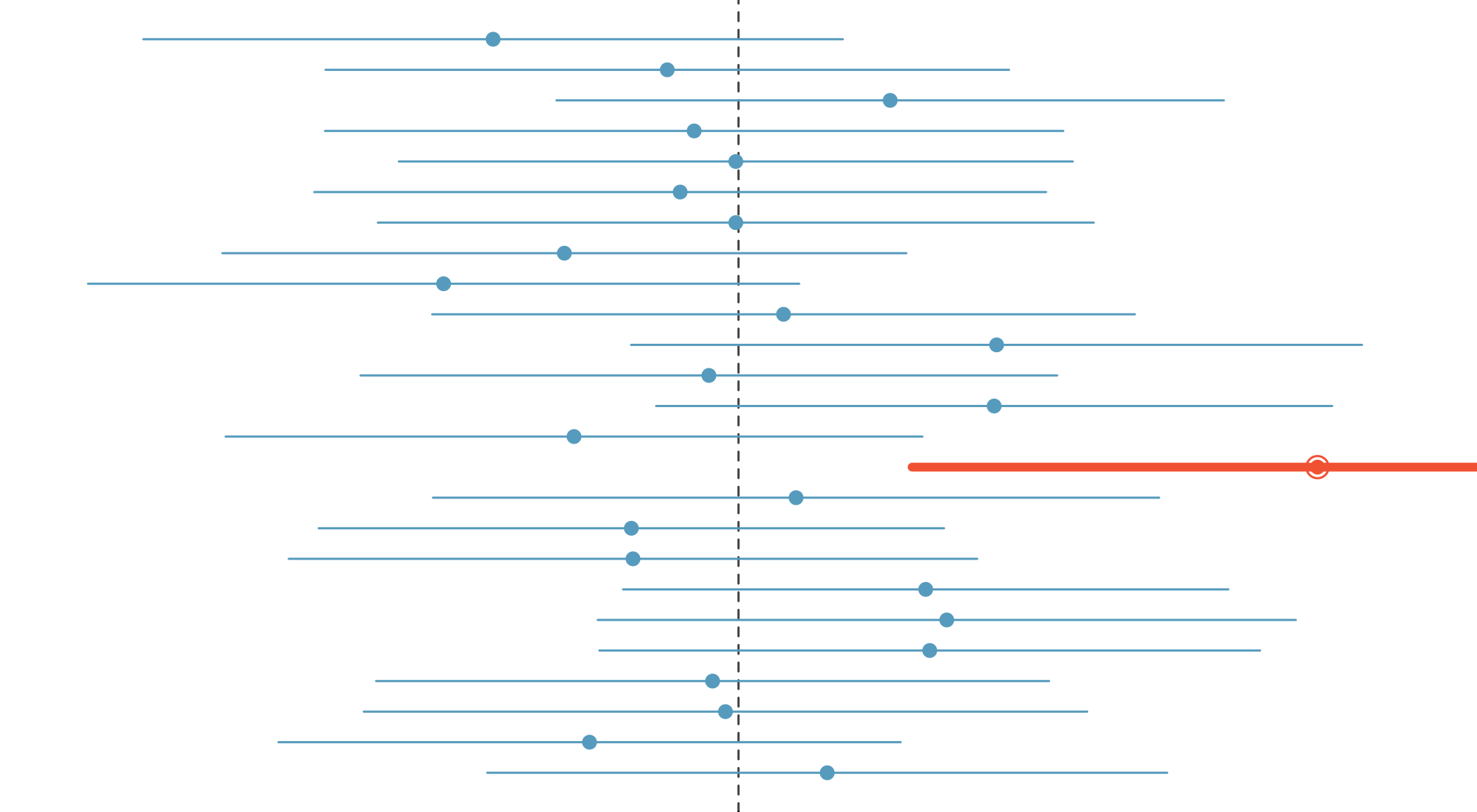
We are 95% confident that …
Confidence intervals identify a plausible range of values for the population parameter…
…they do not identify the probability that the true population parameter falls within the specified range.
Image credit: Figure 17.9 from IMS
#| '!! shinylive warning !!': |
#| shinylive does not work in self-contained HTML documents.
#| Please set `embed-resources: false` in your metadata.
#| label: ci-level
#| viewerHeight: 700
#| viewerWidth: "100%"
#| standalone: true
library(shiny)
# Load only the specific packages needed instead of the entire tidyverse
library(dplyr)
library(ggplot2)
library(tibble)
library(tidyr) # For uncount()
library(infer)
library(bslib)
# Generate the dataset
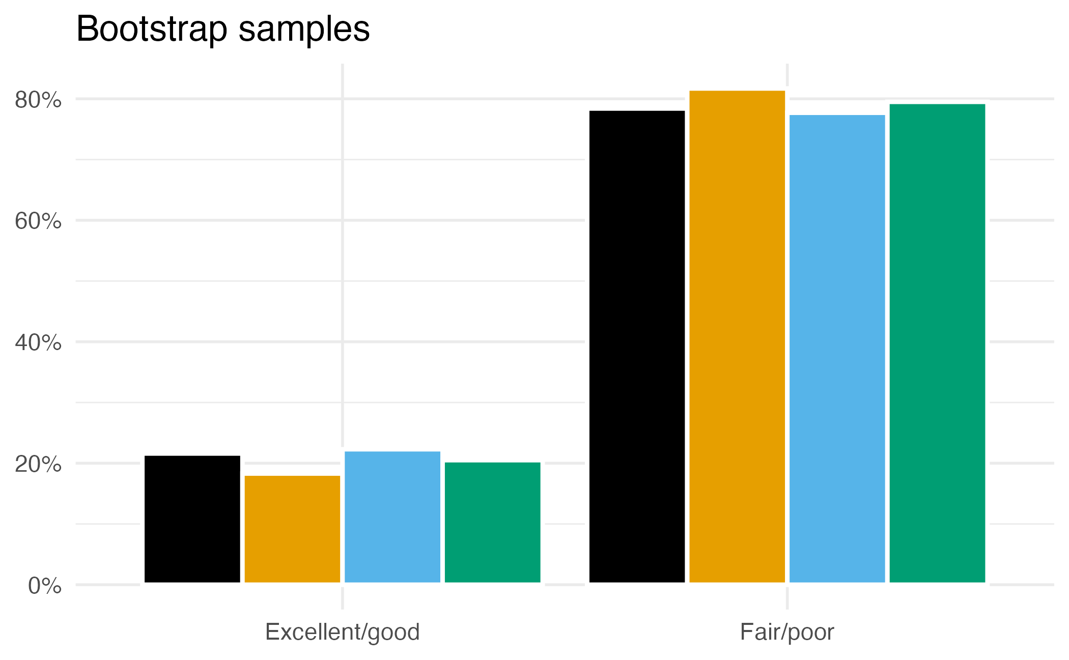
economy <- tribble(
~ response, ~n,
"Excellent/good", 210,
"Fair/poor", 790
) |>
uncount(weights = n)
# Pre-calculate bootstrap distribution to use in the app
set.seed(123)
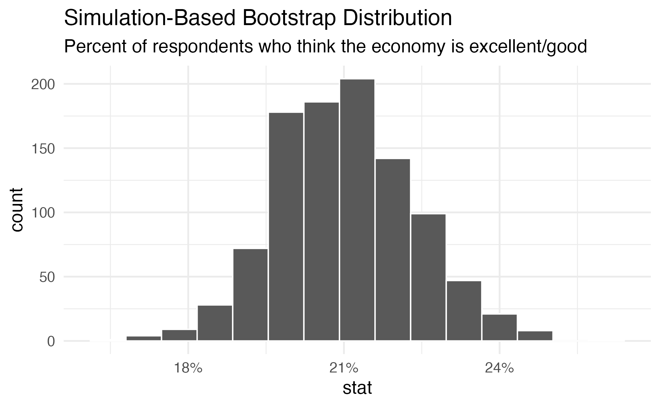
bootstrap_dist <- economy |>
specify(response = response, success = "Excellent/good") |>
generate(reps = 1000, type = "bootstrap") |>
calculate(stat = "prop")
ui <- page_fluid(
title = "Confidence Interval Demo",
tags$style(HTML("
.shiny-input-container .control-label {
font-size: 18px;
font-weight: bold;
}
.irs-min, .irs-max, .irs-single, .irs-from, .irs-to {
font-size: 14px !important;
}
.irs-grid-text {
font-size: 12px !important;
}
")),
sliderInput("conf_level",
"Confidence Level",
min = 0.80,
max = 0.99,
value = 0.95,
step = 0.01,
width = "100%"),
plotOutput("bootstrap_plot", height = "475px")
)
server <- function(input, output) {
# Calculate confidence interval based on the selected confidence level
ci_data <- reactive({
bootstrap_dist |>
get_confidence_interval(level = input$conf_level)
})
# Calculate proportion estimate from original data
observed_prop <- reactive({
economy |>
specify(response = response, success = "Excellent/good") |>
calculate(stat = "prop") |>
pull()
})
# Create bootstrap distribution plot with confidence interval
output$bootstrap_plot <- renderPlot({
conf_level <- input$conf_level
ci <- ci_data()
# Calculate bin width for histogram
bin_width <- (max(bootstrap_dist$stat) - min(bootstrap_dist$stat)) / 30
ggplot(bootstrap_dist, aes(x = stat)) +
geom_histogram(binwidth = bin_width, fill = "skyblue", color = "white", alpha = 0.8) +
geom_vline(xintercept = observed_prop(), color = "red", linewidth = 1.2) +
geom_vline(xintercept = ci$lower_ci, color = "blue", linetype = "dashed", linewidth = 1) +
geom_vline(xintercept = ci$upper_ci, color = "blue", linetype = "dashed", linewidth = 1) +
annotate("rect",
xmin = ci$lower_ci, xmax = ci$upper_ci,
ymin = 0, ymax = Inf,
alpha = 0.2, fill = "blue") +
labs(
title = paste0(conf_level*100, "% Confidence Interval"),
x = "Proportion",
y = "Count"
) +
theme_minimal(base_size = 18) + # Increased base size from 12 to 18
theme(
plot.title = element_text(hjust = 0.5, size = 20), # Increased from 14 to 20
axis.title = element_text(size = 16), # Increased from 10 to 16
axis.text = element_text(size = 14), # Added larger axis text
plot.margin = margin(5, 5, 5, 5)
)
})
}
shinyApp(ui, server)If we want to be very certain that we capture the population parameter, should we use a wider or a narrower interval?
What drawbacks are associated with using a wider interval?

How can we get best of both worlds – high precision and high accuracy?
Related, but have distinct motivations
Confidence interval: range of plausible values for the population parameter
Distribution centered around the observed sample statistic
\(p\)-value: probability of observing the data, given the null hypothesis is true
Distribution centered around the value from the null hypothesis
XX% confidence interval is equivalent to hypothesis test at \(\alpha = 1 - XX\%\)
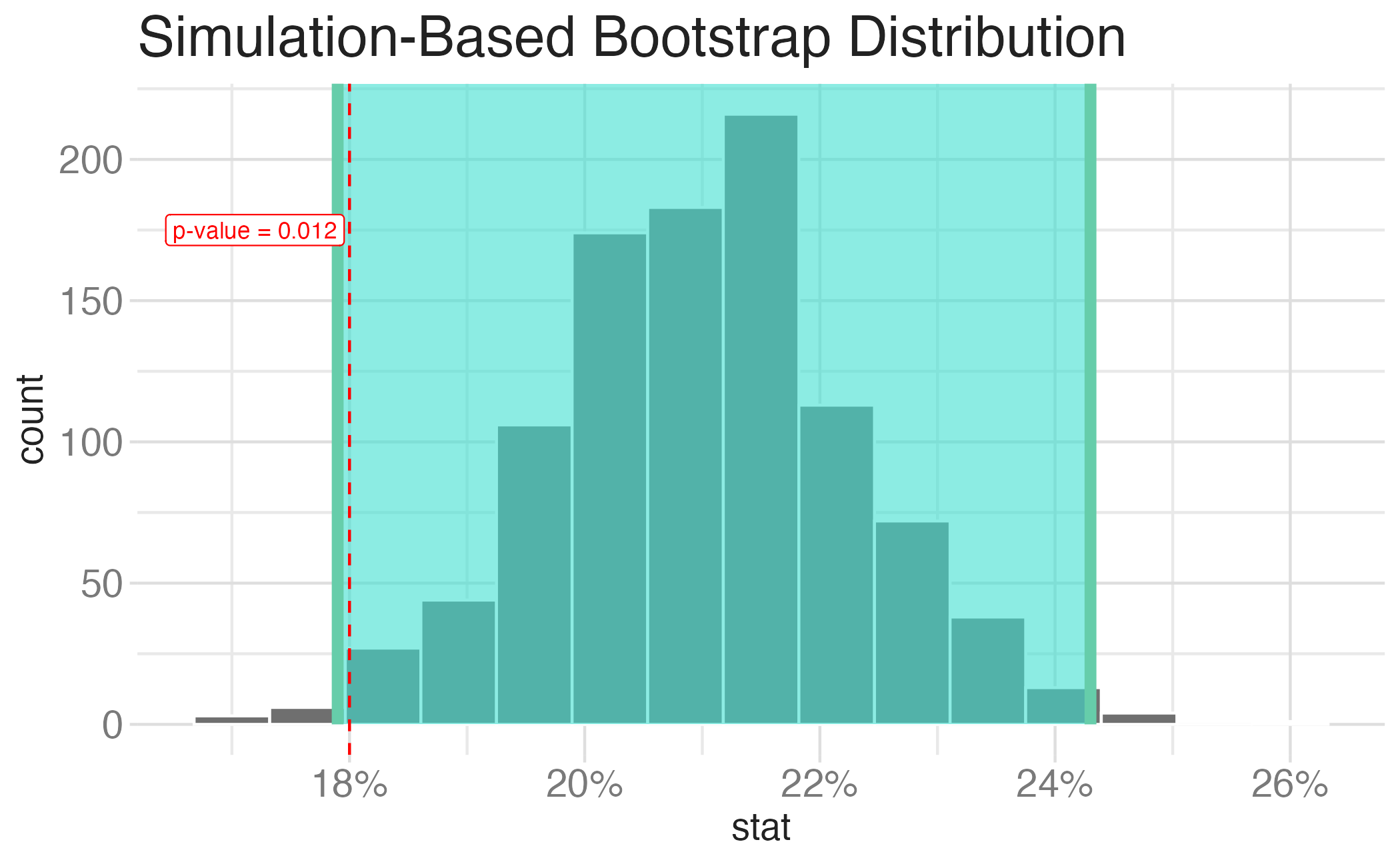
Null hypothesis: The percentage of the American public who believes the economy is excellent/good is 18%.
\[H_0: p = 0.18\]
Alternative hypothesis: The percentage of the American public who believes the economy is excellent/good is different from 18%.
\[H_A: p \neq 0.18\]
Source: Gio Circo
ae-15Instructions
ae-15 (repo name will be suffixed with your GitHub name).renv::restore() to install the required packages, open the Quarto document in the repo, and follow along and complete the exercises.calculate(stat = "mean")calculate(stat = "median")fit()