AE 03: Joining prognosticators

Application exercise

Modified

February 3, 2026

Important

Go to the course GitHub organization and locate the repo titled ae-03-YOUR_GITHUB_USERNAME to get started.

This AE is due February 3 at 11:59pm.

library(tidyverse)
library(scales)
library(feb2)

Prognosticator success

Every year on February 2, Groundhog Day, the famous groundhog Punxsutawney Phil—and a growing cast of creatures (including stuffed animals, sock puppets, and mascots)—emerge from their burrows to predict the weather. Punxsutawney Phil, the prognosticator of prognosticators, has been predicting the weather since 1887. If he sees his shadow, his prediction is for six more weeks of winter. If not, he predicts an early spring.

Over time the number of prognosticators across the country has grown to over 150. {feb2} collects and collates data on these prognisticators, their predictions, and importantly their performance. Do these prognosticators have any skill? Does that vary whether or not they be animal, inanimate, or humans dressed as animals?

In this exercise, we will use data from {feb2} and weather data from NOAA to evaluate prognosticator skill.

Load the data

{feb2} partitions the data into three data frames: class_def1, prognosticators, and predictions.

Let’s take a look at the data frames.

glimpse(class_def1)

Rows: 15,976
Columns: 3
$ prognosticator_city <chr> "02", "02", "02", "02", "02", "02", "02", "02", "0…
$ year                <dbl> 1926, 1927, 1928, 1929, 1930, 1931, 1932, 1933, 19…
$ class               <chr> NA, NA, NA, NA, NA, NA, NA, NA, NA, NA, NA, NA, NA…

glimpse(prognosticators)

Rows: 315
Columns: 14
$ prognosticator_name      <chr> "Punxsutawney Phil", "Octoraro Orphie", "Poor…
$ Status                   <chr> "Active", "Active", "Active", "Deceased", "Ac…
$ prognosticator_slug      <chr> "Punxsutawney-Phil", "Octoraro-Orphie", "Poor…
$ prognosticator_type_orig <chr> "Groundhog", "Taxidermy mount Groundhog", "St…
$ prognosticator_city      <chr> "Punxsutawney, PA", "Quarryville, PA", "York,…
$ `Last Prediction`        <chr> "2025", "2025", "2025", "1948", "1954", "1961…
$ prognosticator_lat       <dbl> 40.94363, 39.89705, 39.96249, 39.95272, 39.95…
$ prognosticator_long      <dbl> -78.97108, -76.16357, -76.72770, -75.16353, -…
$ prognosticator_type      <chr> "Groundhog", "Stuffed Groundhog", "Stuffed Gr…
$ prognosticator_status    <chr> "Creature", "Inanimate", "Inanimate", "Creatu…
$ prognosticator_creature  <chr> "Groundhog", "Groundhog", "Groundhog", "Groun…
$ prognosticator_phylum    <chr> "Chordata", "Chordata", "Chordata", "Chordata…
$ prognosticator_class     <chr> "Mammalia", "Mammalia", "Mammalia", "Mammalia…
$ prognosticator_order     <chr> "Rodentia", "Rodentia", "Rodentia", "Rodentia…

glimpse(predictions)

Rows: 2,482
Columns: 6
$ prognosticator_name  <chr> "Punxsutawney Phil", "Punxsutawney Phil", "Punxsu…
$ prognosticator_slug  <chr> "Punxsutawney-Phil", "Punxsutawney-Phil", "Punxsu…
$ year                 <int> 1887, 1888, 1889, 1890, 1891, 1892, 1893, 1894, 1…
$ prediction_orig      <chr> "Long Winter", "Long Winter", "No Record", "Early…
$ prediction           <chr> "Long Winter", "Long Winter", NA, "Early Spring",…
$ predict_early_spring <int> 0, 0, NA, 1, NA, NA, NA, NA, NA, NA, NA, 0, NA, 0…

Your turn: Identify the primary key variable(s) for each data frame. What is each data frame’s foreign key variable(s) that can be used to join the data frames together?

Look up the documentation for each data frame

You can access documentation for each of the data frames by using the ? operator in the R console

?class_def1

`class_def1`

Primary key variable(s): Add response here.

Foreign key variable(s)

prognosticators: Add response here.
predictions: Add response here.

`prognosticators`

Primary key variable(s): Add response here.

Foreign key variable(s)

class_def1: Add response here.
predictions: Add response here.

`predictions`

Primary key variable(s): Add response here.

Foreign key variable(s)

class_def1: Add response here.
prognosticators: Add response here.

Join the data frames

Your turn: Join the three data frames using an appropriate sequence of *_join() functions and assign the joined data frame to seers_weather.

# add code here

Calculate the variables

Demo: Take a look at the updated seers data frame. First we need to calculate for each prediction whether or not the prognostication was correct.

# add code here

Demo: Calculate the accuracy rate (we’ll call it preds_rate) for weather predictions using the summarize() function in {dplyr}. Note that the function for calculating the mean is mean() in R.

# add code here

Your turn (5 minutes): Now expand your calculations to also calculate the number of predictions in each region and the standard error of accuracy rate. Store this data frame as seers_summary. Recall the formula for the standard error of a sample proportion:

\[SE(\hat{p}) \approx \sqrt{\frac{(\hat{p})(1 - \hat{p})}{n}}\]

# add code here

Demo: Take the seers_summary data frame and order the results in descending order of accuracy rate.

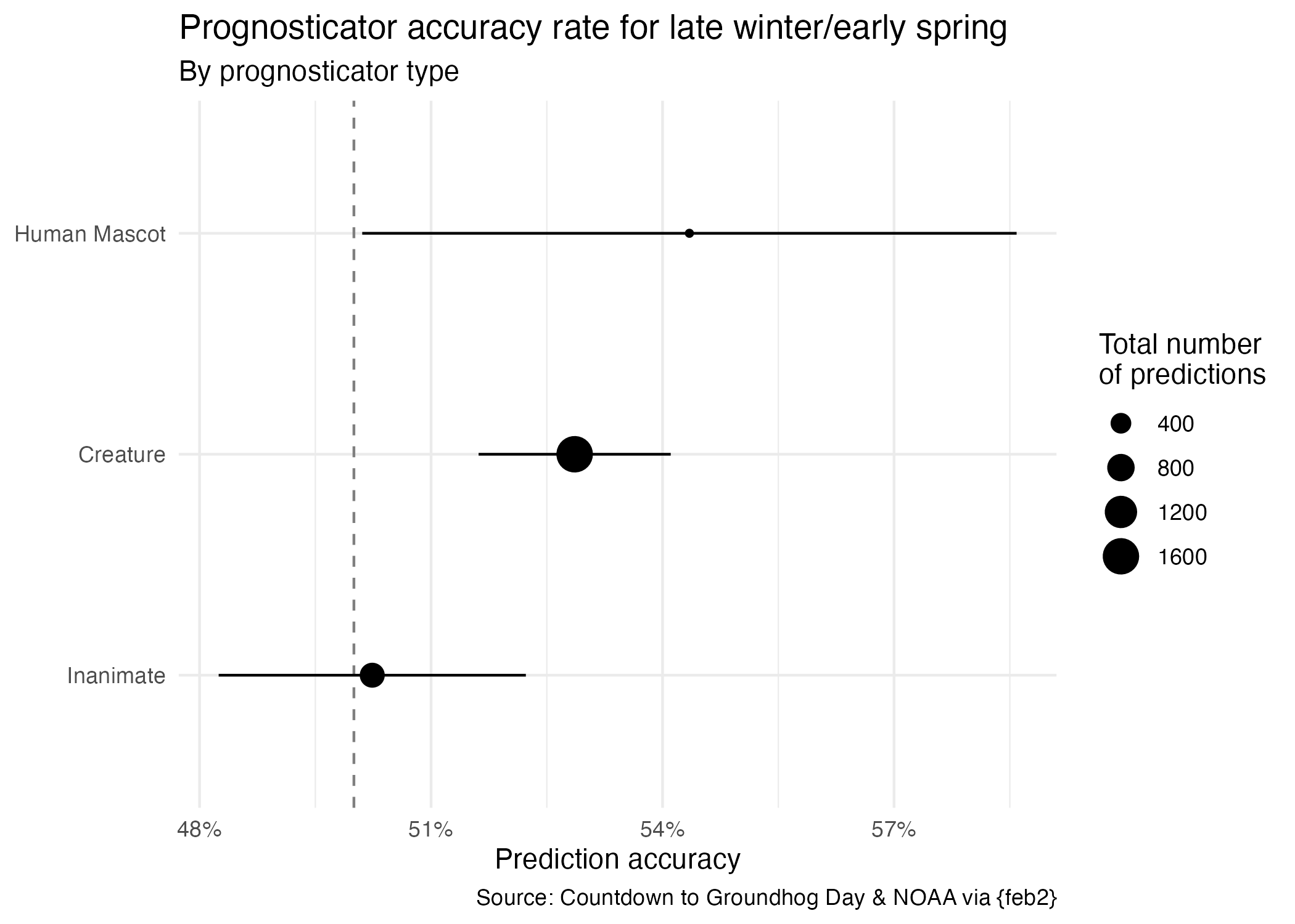
# add code here

Recreate the plot

Demo: Recreate the following plot using the data frame you have developed so far.

# add code here
seers_summary |>
  mutate(
    prognosticator_status = fct_reorder(
      .f = ______,
      .x = ______
    )
  ) |>
  ggplot(mapping = aes(x = preds_rate, y = prognosticator_status)) +
  geom_vline(xintercept = 0.5, linetype = "dashed", color = "gray50") +
  geom_point(mapping = aes(size = preds_n)) +
  geom_linerange(
    mapping = aes(
      xmin = ______,
      xmax = ______
    )
  ) +
  scale_x_continuous(labels = label_percent()) +
  labs(
    title = "Prognosticator accuracy rate for late winter/early spring",
    subtitle = "By prognosticator type",
    x = "Prediction accuracy",
    y = NULL,
    size = "Total number\nof predictions",
    caption = "Source: Countdown to Groundhog Day & NOAA via {feb2}"
  ) +
  theme_minimal()

Error in parse(text = input): <text>:5:13: unexpected input
4:     prognosticator_status = fct_reorder(
5:       .f = __
               ^

Your turn (time permitting): Make any other changes you would like to improve it.

# add your code here